Simulating EBSD data
How to simulate an arbitrary number of individual orientations data from any ODF.
| On this page ... |
| Simulate EBSD Data |
| ODF Estimation from EBSD Data |
| Exploration of the relationship between estimation error and number of single orientations |
MTEX allows one to simulate an arbitrary number of EBSD data from any ODF. This is quite helpful if you want to analyze the EBSD to ODF estimation routine.
Define a Model ODF
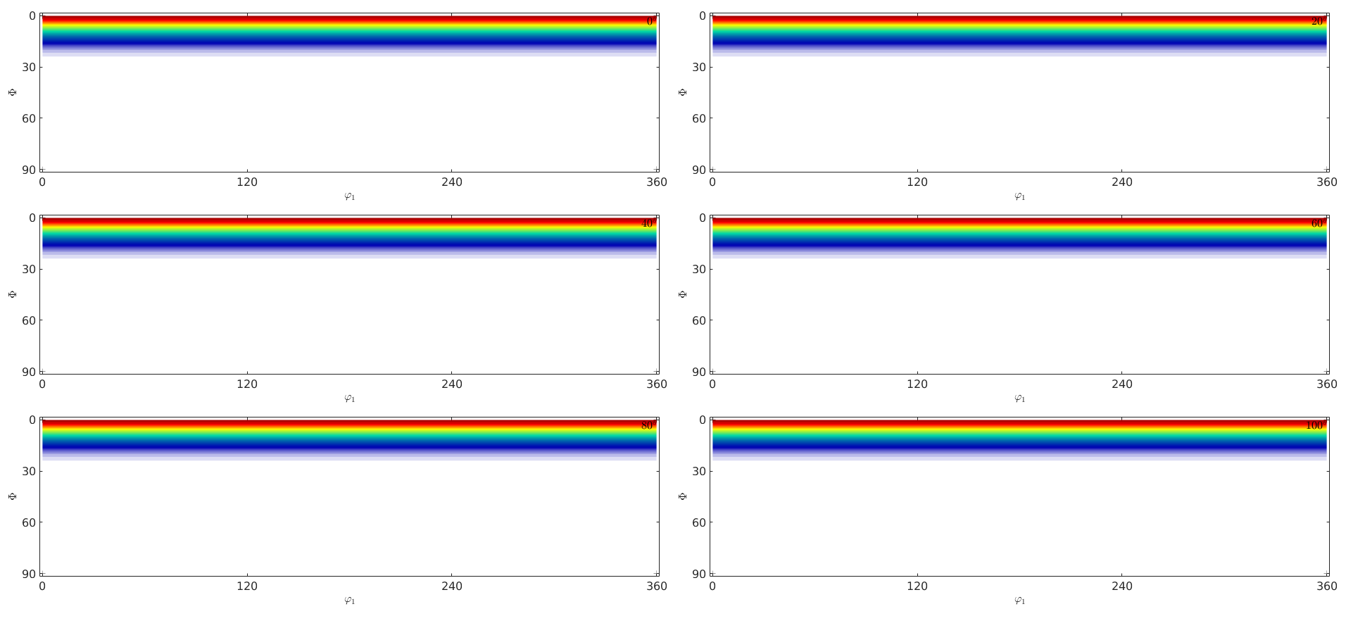
Let us first define a simple fibre symmetric ODF.
cs = crystalSymmetry('32');
fibre_odf = 0.5*uniformODF(cs) + 0.5*fibreODF(Miller(0,0,0,1,cs),zvector);plot(fibre_odf,'sections',6,'silent')
Warning: Plot properties not compatible to previous plot! I'going to create a
new figure.
Simulate EBSD Data
This ODF we use now to simulate 10000 individual orientations.
ori = calcOrientations(fibre_odf,10000)
ori = orientation
  size: 10000 x 1
  crystal symmetry : 321, X||a*, Y||b, Z||c*
  specimen symmetry: 1
ODF Estimation from EBSD Data
From the 10000 individual orientations, we can now estimate an ODF. First, we determine the optimal kernel function
psi = calcKernel(ori)
psi = deLaValleePoussinKernel
  bandwidth: 43
  halfwidth: 5.7°
and then we use this kernel function for kernel density estimation
odf = calcODF(ori,'kernel',psi)
odf = ODF
  crystal symmetry : 321, X||a*, Y||b, Z||c*
  specimen symmetry: 1

  Harmonic portion:
    degree: 43
    weight: 1
which can be plotted,
plot(odf,'sections',6,'silent')
Warning: Plot properties not compatible to previous plot! I'going to create a
new figure.
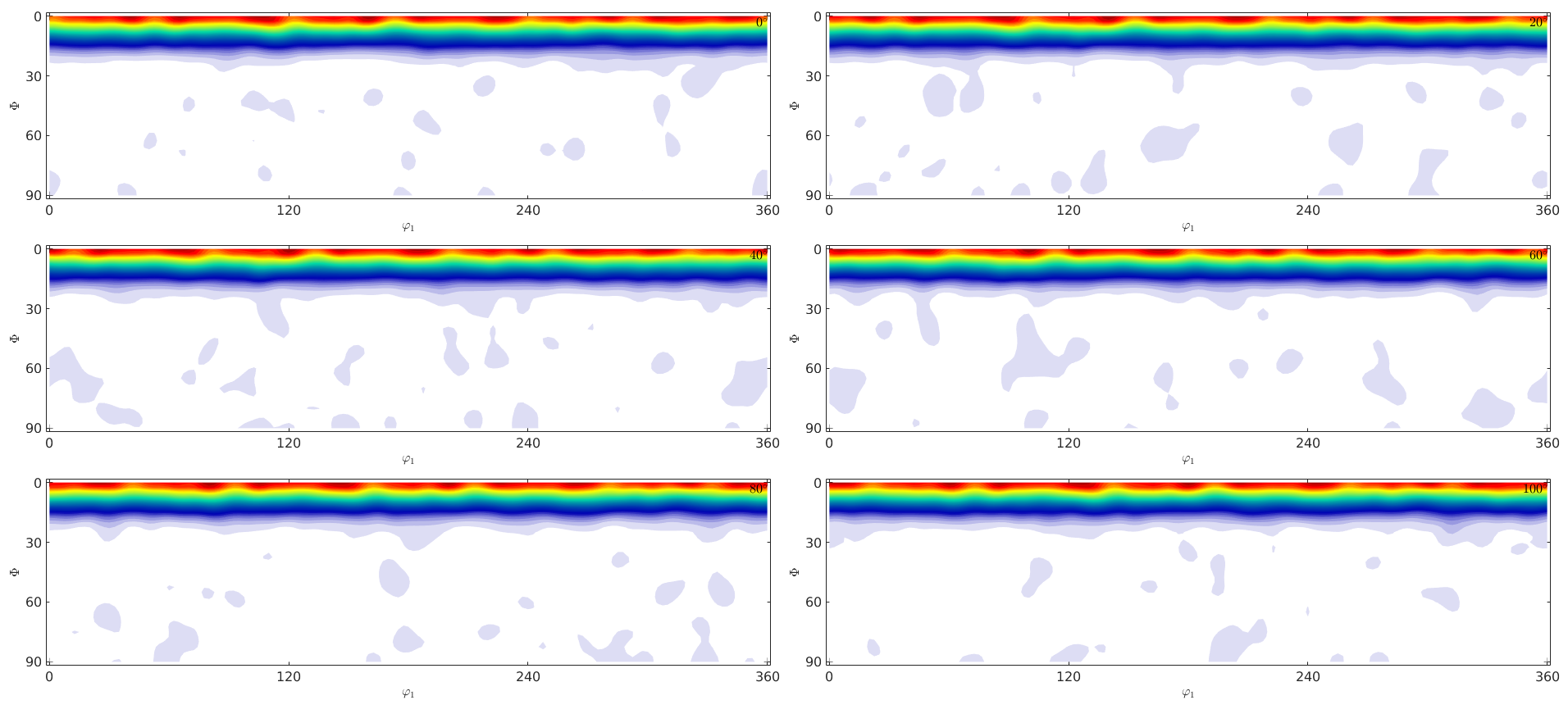
and compared to the original model ODF.
calcError(odf,fibre_odf,'resolution',5*degree)ans =
0.0947
Exploration of the relationship between estimation error and number of single orientations
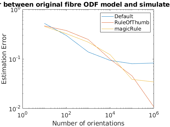
For a more systematic analysis of the estimation error, we simulate 10, 100, ..., 1000000 single orientations of the model ODF and calculate the approximation error for the ODFs estimated from these data.
e = [];
for i = 1:6

  ori = calcOrientations(fibre_odf,10^i,'silent');

  psi1 = calcKernel(ori,'SamplingSize',10000,'silent');
  odf = calcODF(ori,'kernel',psi1,'silent');
  e(i,1) = calcError(odf,fibre_odf,'resolution',2.5*degree);

  psi2 = calcKernel(ori,'method','RuleOfThumb','silent');
  odf = calcODF(ori,'kernel',psi2,'silent');
  e(i,2) = calcError(odf,fibre_odf,'resolution',2.5*degree);

  psi3 = calcKernel(ori,'method','magicRule','silent');
  odf = calcODF(ori,'kernel',psi3,'silent');
  e(i,3) = calcError(odf,fibre_odf,'resolution',2.5*degree);

  disp(['RuleOfThumb: ' int2str(psi2.halfwidth/degree) mtexdegchar ...
    ' KLCV: ' int2str(psi1.halfwidth/degree) mtexdegchar ...
    ' magicRule: ' int2str(psi3.halfwidth/degree) mtexdegchar ...
    ]);

end
RuleOfThumb: 26° KLCV: 12° magicRule: 31°
RuleOfThumb: 37° KLCV: 15° magicRule: 22°
RuleOfThumb: 19° KLCV: 9° magicRule: 16°
RuleOfThumb: 10° KLCV: 6° magicRule: 11°
RuleOfThumb: 9° KLCV: 5° magicRule: 8°
RuleOfThumb: 7° KLCV: 4° magicRule: 6°
Plot the error in dependency of the number of single orientations.
close all;
loglog(10.^(1:length(e)),e)
legend('Default','RuleOfThumb','magicRule')
xlabel('Number of orientations')
ylabel('Estimation Error')
title('Error between original fibre ODF model and simulated ebsd','FontWeight','bold')
| DocHelp 0.1 beta |