Crystal Shapes (The Class crystalShape)

How to draw threedimensional representations of crystals.

Simple Crystal Shapes

Calculating with crystal shapes

Plotting crystal shapes

Twinning relationships

Defining complicated crystal shapes

Marking crystal faces

Defining complicated crystals more simple

Select Faces

Gallery of hardcoded crystal shapes

Complete Function list

Simple Crystal Shapes

In the case of cubic or hexagonal materials the corresponding crystal are often represented as cubes or hexagons, where the faces correspond to the lattice planes {100} in the cubic case and {1,0,-1,0},{0,0,0,1} in the hexagonal case. Such simplifies crystal shapes may be created in MTEX with the commands

% import some hexagonal data
mtexdata titanium;

% define a simple hexagonal crystal shape
cS = crystalShape.hex(ebsd.CS)

% and plot it
close all
plot(cS)

 loading data ...
 saving data to /home/hielscher/mtex/master/data/titanium.mat
 
cS = crystalShape  
 mineral: Titanium (Alpha) (622, X||a, Y||b*, Z||c)
 vertices: 12
 faces: 8

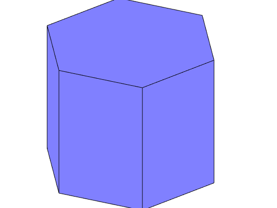
Internally, a crystal shape is represented as a list of faces which are bounded by a list of vertices

cS.V

 
ans = vector3d  
 size: 12 x 1
          x         y         z
  -0.393614         0 -0.308331
  -0.393614         0  0.308331
  -0.196807  -0.34088  0.308331
  -0.196807   0.34088 -0.308331
  -0.196807  -0.34088 -0.308331
  -0.196807   0.34088  0.308331
   0.196807  -0.34088  0.308331
   0.196807   0.34088 -0.308331
   0.196807  -0.34088 -0.308331
   0.196807   0.34088  0.308331
   0.393614         0 -0.308331
   0.393614         0  0.308331

Calculating with crystal shapes

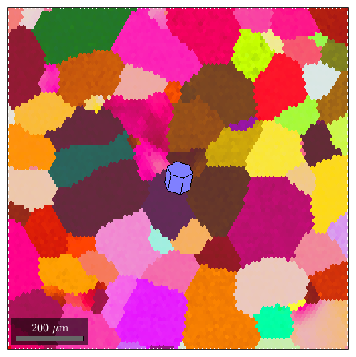
Crystal shapes are defined in crystal coordinates. Thus applying an orientation rotates them into specimen coordinates. This functionality can be used to visualize crystal orientations in EBSD maps

% plot an EBSD map
clf % clear current figure
plot(ebsd,ebsd.orientations)

hold on
scaling = 100; % scale the crystal shape to have a nice size

% plot at position (500,500) the orientatation of the corresponding crystal
plot(500,500,50, ebsd(500,500).orientations * cS * scaling)
hold off

Warning: Possibly applying an orientation to an object in specimen coordinates!

As we have seen in the previous section we can apply several operations on crystal shapes. These include

factor * cS scales the crystal shape in size
ori * cS rotates the crystal shape in the defined orientation
[xy] + cS or [xyz] + cS shifts the crystal shape in the specified positions

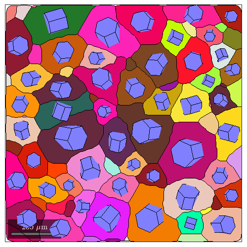
At this point it comes into help that MTEX supports lists of crystal shapes, i.e., whenever one of the operations listed above includes a list (e.g. a list of orientations) the multiplication will yield a list of crystal shapes. Lets illustrate this

% compute some grains
grains = calcGrains(ebsd);
grains = smooth(grains,5);

% and plot them
plot(grains,grains.meanOrientation)

% find the big ones
isBig = grains.grainSize>50;

% define a list of crystal shape that is oriented as the grain mean
% orientation and scaled according to their area
cSGrains = grains(isBig).meanOrientation * cS * 0.7 * sqrt(grains(isBig).area);

% now we can plot these crystal shapes at the grain centers
hold on
plot(grains(isBig).centroid + cSGrains)
hold off

  I'm going to colorize the orientation data with the 
  standard MTEX colorkey. To view the colorkey do:
 
  colorKey = ipfColorKey(ori_variable_name)
  plot(colorKey)
Warning: Possibly applying an orientation to an object in specimen coordinates!

Plotting crystal shapes

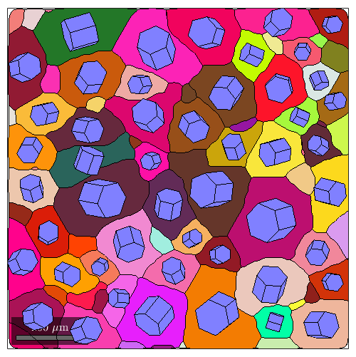
The above can be accomplished a bit more directly and a bit more nice with

% plot a grain map
plot(grains,grains.meanOrientation)

% and on top for each large grain a crystal shape
hold on
plot(grains(isBig),0.7*cS)
hold off

  I'm going to colorize the orientation data with the 
  standard MTEX colorkey. To view the colorkey do:
 
  colorKey = ipfColorKey(ori_variable_name)
  plot(colorKey)
Warning: Possibly applying an orientation to an object in specimen coordinates!

In the same manner we may visualize grain orientations and grains size within pole figures

plotPDF(grains(isBig).meanOrientation,Miller({1,0,-1,0},{0,0,0,1},ebsd.CS),'contour')
plot(grains(isBig).meanOrientation,0.002*cSGrains,'add2all')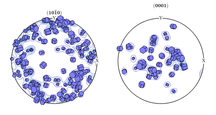

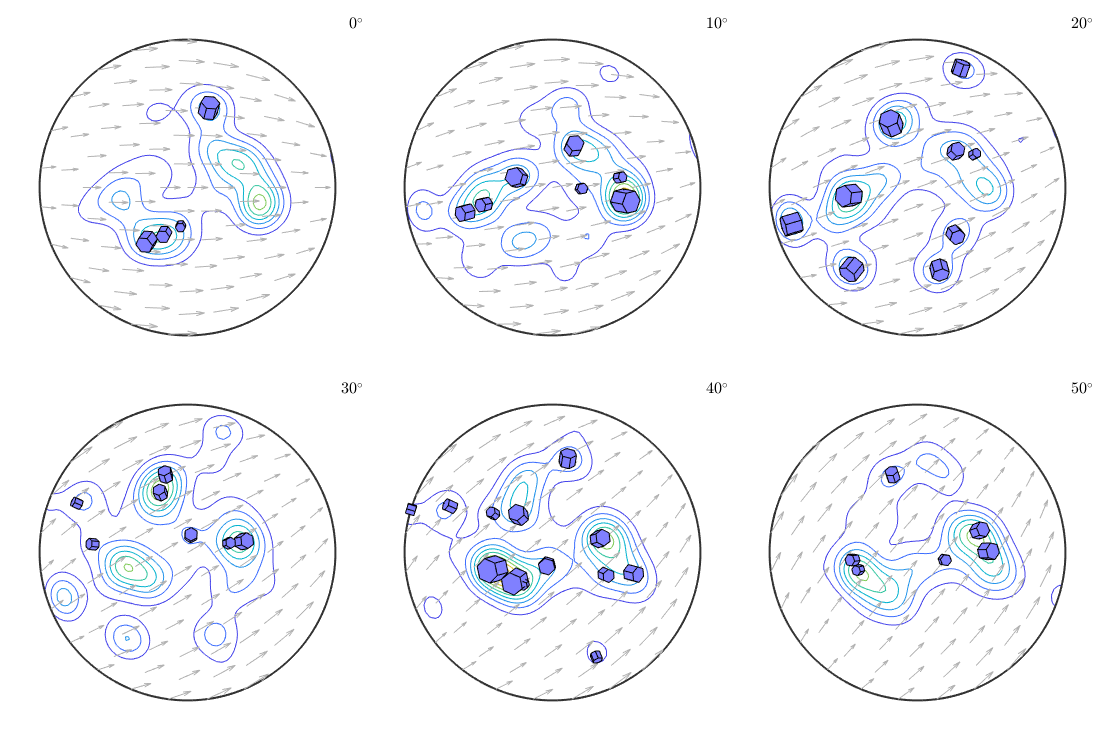
or even within ODF sections

% compute the odf
odf = calcODF(ebsd.orientations);

% plot the odf in sigma sections
plotSection(odf,'sigma','contour')

% and on top of it the crystal shapes
plot(grains(isBig).meanOrientation,0.002*cSGrains,'add2all')

Twinning relationships

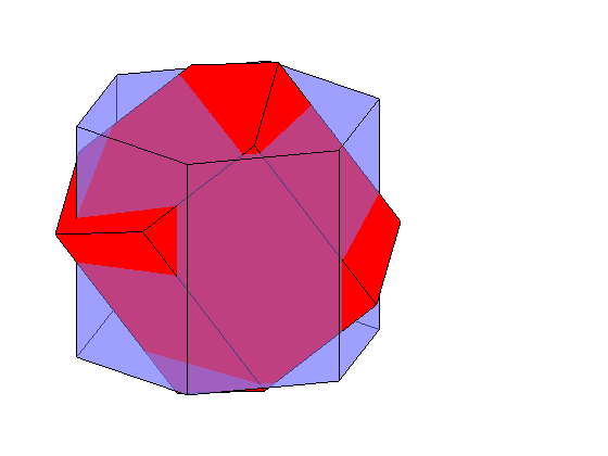
We may also you crystal shapes to illustrate twinning relation ships

% define some twinning misorientation
mori = orientation.byAxisAngle(Miller({1 0-1 0},ebsd.CS),34.9*degree)

% plot the crystal in ideal orientation
close all
plot(cS,'FaceAlpha',0.5)

% and on top of it in twinning orientation
hold on
plot(mori * cS *0.9,'FaceColor','r')
hold off
view(45,20)

 
mori = misorientation  
  size: 1 x 1
  crystal symmetry : Titanium (Alpha) (622, X||a, Y||b*, Z||c)
  crystal symmetry : Titanium (Alpha) (622, X||a, Y||b*, Z||c)
 
  Bunge Euler angles in degree
  phi1  Phi phi2 Inv.
   330 34.9   30    0
 
Warning: Possibly applying an orientation to an object in specimen coordinates!

Defining complicated crystal shapes

For symmetries other then hexagonal or cubic one would like to have more complicated crystal shape representing the true appearance. To this end one has to include more faces into the representation and carefuly adjust their distance to the origin.

Lets consider a quartz crystal.

cs = loadCIF('quartz')

 
cs = crystalSymmetry  
 
  mineral        : Quartz            
  symmetry       : 321               
  a, b, c        : 4.9, 4.9, 5.4     
  reference frame: X||a*, Y||b, Z||c*

Its shape is mainly bounded by the following faces

m = Miller({1,0,-1,0},cs);  % hexagonal prism
r = Miller({1,0,-1,1},cs);  % positive rhomboedron, usally bigger then z
z = Miller({0,1,-1,1},cs);  % negative rhomboedron
s1 = Miller({2,-1,-1,1},cs);% left tridiagonal bipyramid
s2 = Miller({1,1,-2,1},cs); % right tridiagonal bipyramid
x1 = Miller({6,-1,-5,1},cs);% left positive Trapezohedron
x2 = Miller({5,1,-6,1},cs); % right positive Trapezohedron

If we take only the first three faces we end up with

N = [m,r,z];
cS = crystalShape(N)

plot(cS)

 
cS = crystalShape  
 mineral: Quartz (321, X||a*, Y||b, Z||c*)
 vertices: 8
 faces: 18

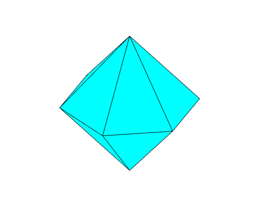
i.e. we see only the possitive and negative rhomboedrons, but the hexagonal prism are to far away from the origin to cut the shape. We may decrease the distance, by multiplying the coresponding normal with a factor larger then 1.

N = [2*m,r,z];

cS = crystalShape(N);
plot(cS)

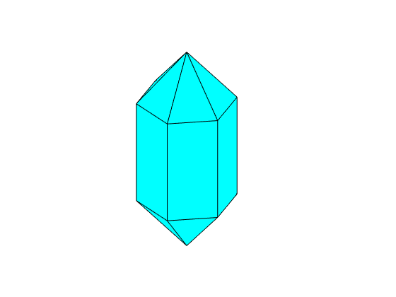
Next in a typical Quartz crystal the negativ rhomboedron is a bit smaller then the positiv rhomboedron. Lets correct for this.

% collect the face normal with the right scalling
N = [2*m,r,0.9*z];

cS = crystalShape(N);
plot(cS)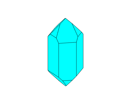

Finaly, we add the tridiagonal bipyramid and the positive Trapezohedron

% collect the face normal with the right scalling
N = [2*m,r,0.9*z,0.7*s1,0.3*x1];

cS = crystalShape(N);
plot(cS)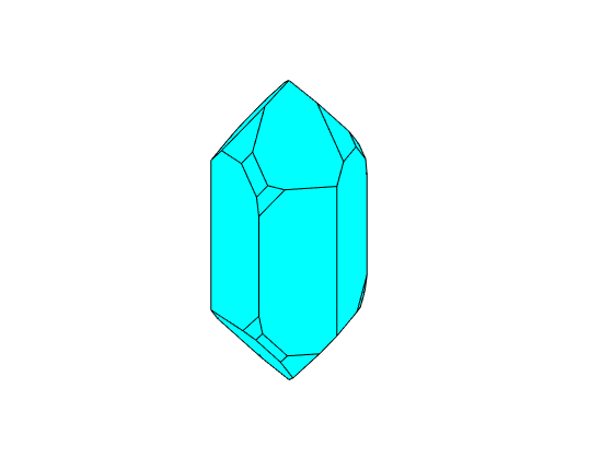

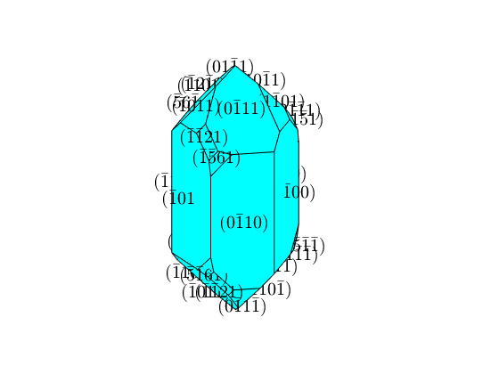
Marking crystal faces

We may colorize the faces according to their lattice planes using the command

plot(cS,'colored')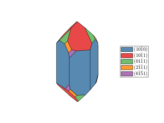

or even label the faces directly

plot(cS)
N = unique(cS.N.symmetrise,'noSymmetry','stable');
fC = cS.faceCenter;

for i = 1:length(N)
  text3(fC(i),char(round(N(i)),'latex'),'scaling',1.1,'interpreter','latex')
end

Defining complicated crystals more simple

We see that defining a complicated crystal shape is a tedious work. To this end MTEX allows to model the shape with a habitus and a extension parameter. This approach has been developed by J�rg Enderlein in Enderlein, J., 1997. A package for displaying crystal morphology. Mathematica Journal, 7(1). The two paraters are used to model the distance of a phase from the origin. Setting all parameters to one we obtain

% take the face normals unscaled
N = [m,r,z,s2,x2];

habitus = 1;
extension = [1 1 1];
cS = crystalShape(N,habitus,extension);
plot(cS,'colored')

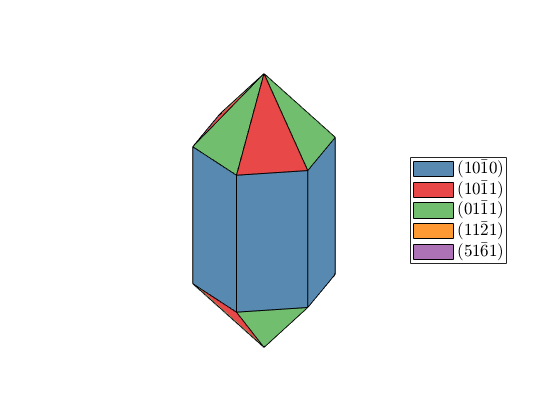
The scale parameter models the inverse extension of the crystal in each dimension. In order to make the crystal a bit longer and the negative rhomboedrons smaller we could do

extension = [0.9 1.1 1];
cS = crystalShape(N,habitus,extension);
plot(cS,'colored')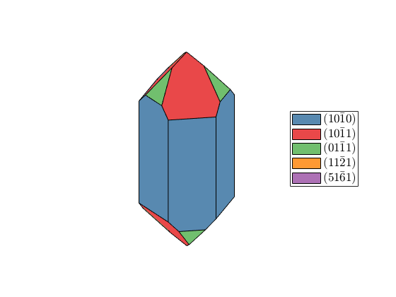

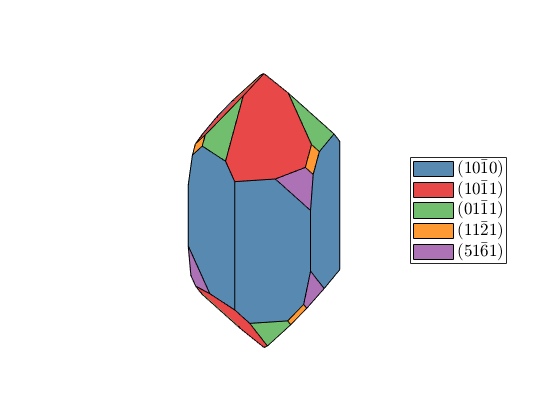
Next the habitus parameter describes how close faces with mixed hkl are to the origin. If we increase the habitus parameter the trapezohedron and the bipyramid become more and more dominant

habitus = 1.1;
cS = crystalShape(N,habitus,extension);
plot(cS,'colored'), snapnow

habitus = 1.2;
cS = crystalShape(N,habitus,extension);
plot(cS,'colored'), snapnow

habitus = 1.3;
cS = crystalShape(N,habitus,extension);
plot(cS,'colored')

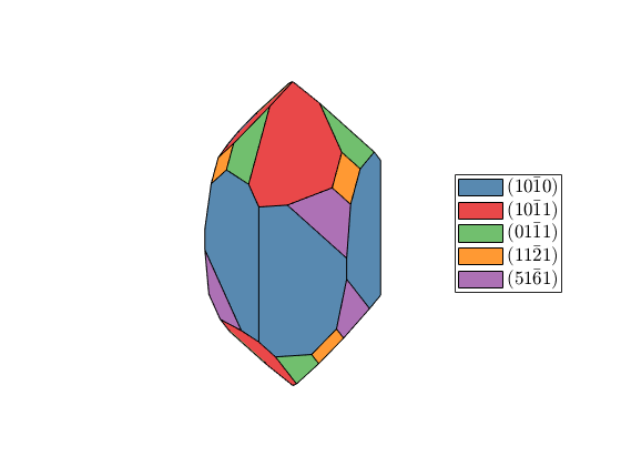
Select Faces

Gallery of hardcoded crystal shapes

plot(crystalShape.olivine,'colored')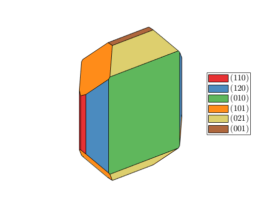

plot(crystalShape.garnet,'colored')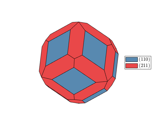

plot(crystalShape.topaz,'colored')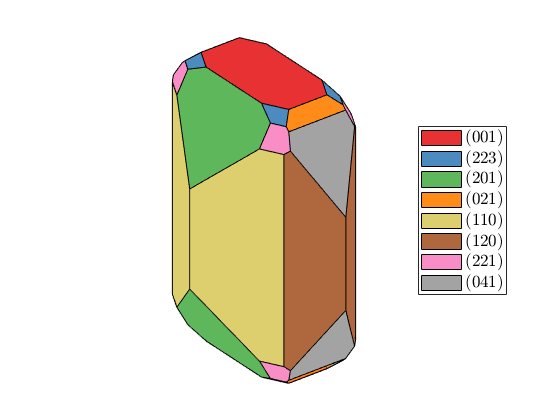

Complete Function list


`The code of this class is based on the paper`

`Enderlein, J., 1997. A package for displaying crystal morphology.`
`Mathematica Journal, 7(1).`

`we need more :)`