Visualizing ODFs

Explains all possibilities to visualize ODfs, i.e. pole figure plots, inverse pole figure plots, ODF sections, fibre sections.

Pole Figures

Inverse Pole Figures

ODF Sections

Plotting the ODF along a fibre

Fourier Coefficients

Axis / Angle Distribution

Let us first define some model ODFs to be plotted later on.

cs = crystalSymmetry('32');
mod1 = orientation.byEuler(90*degree,40*degree,110*degree,'ZYZ',cs);
mod2 = orientation.byEuler(50*degree,30*degree,-30*degree,'ZYZ',cs);

odf = 0.2*unimodalODF(mod1) ...
  + 0.3*unimodalODF(mod2) ...
  + 0.5*fibreODF(Miller(0,0,1,cs),vector3d(1,0,0),'halfwidth',10*degree)

%odf = 0.2*unimodalODF(mod2)

 
odf = ODF  
  crystal symmetry : 321, X||a*, Y||b, Z||c*
  specimen symmetry: 1
 
  Radially symmetric portion:
    kernel: de la Vallee Poussin, halfwidth 10°
    center: (180°,40°,20°)
    weight: 0.2
 
  Radially symmetric portion:
    kernel: de la Vallee Poussin, halfwidth 10°
    center: (140°,30°,240°)
    weight: 0.3
 
  Fibre symmetric portion:
    kernel: de la Vallee Poussin, halfwidth 10°
    fibre: (0001) - 1,0,0
    weight: 0.5

and lets switch to the LaboTex colormap

setMTEXpref('defaultColorMap',LaboTeXColorMap);

Pole Figures

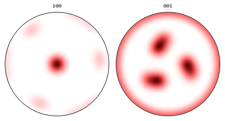
Plotting some pole figures of an ODF is straight forward using the plotPDF command. The only mandatory arguments are the ODF to be plotted and the Miller indice of the crystal directions you want to have pole figures for.

plotPDF(odf,Miller({1,0,-1,0},{0,0,0,1},{1,1,-2,1},cs))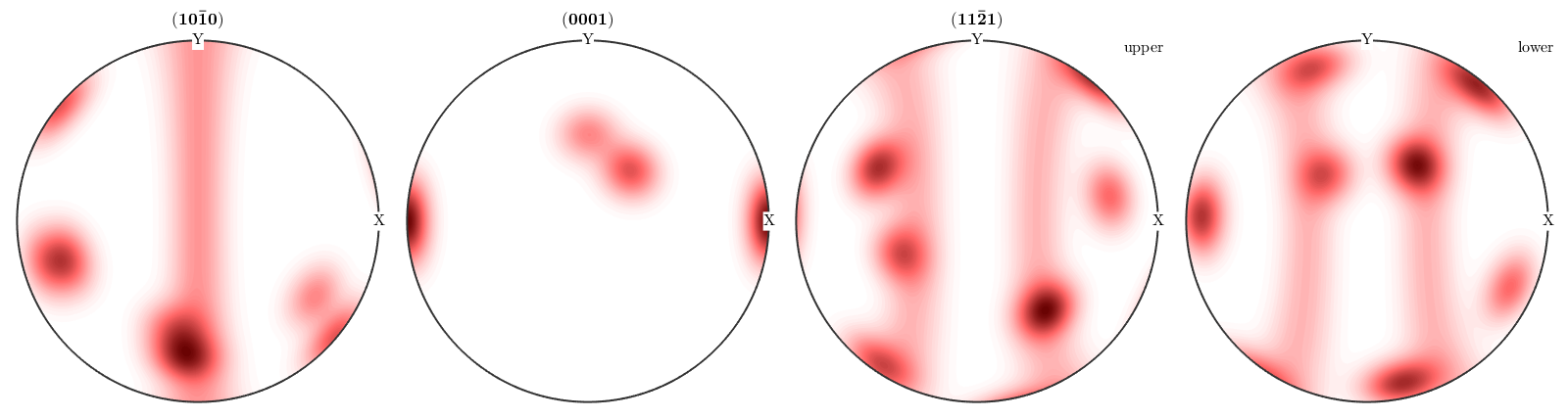

While the first two pole figures are plotted on the upper hemisphere only the (11-21) has been plotted for the upper and lower hemisphere. The reason for this behaviour is that MTEX automatically detects that the first two pole figures coincide on the upper and lower hemisphere while the (11-21) pole figure does not. In order to plot all pole figures with upper and lower hemisphere we can do

plotPDF(odf,Miller({1,0,-1,0},{0,0,0,1},{1,1,-2,1},cs),'complete')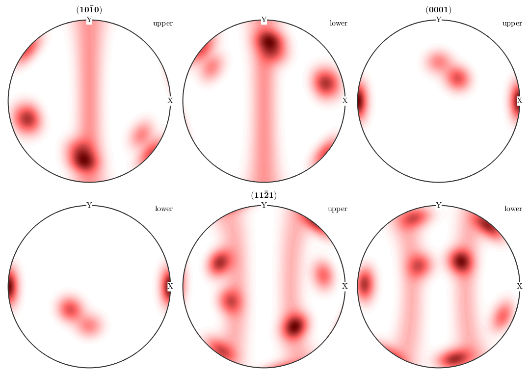

We see that in general upper and lower hemisphere of the pole figure do not coincide. This is only the case if one one following reason is satisfied

the crystal direction h is symmetrically equivalent to -h, in the present example this is true for the c-axis h = (0001)
the symmetry group contains the inversion, i.e., it is a Laue group
we consider experimental pole figures where we have antipodal symmetry, due to Friedel's law.

In MTEX antipodal symmetry can be enforced by the use the option antipodal.

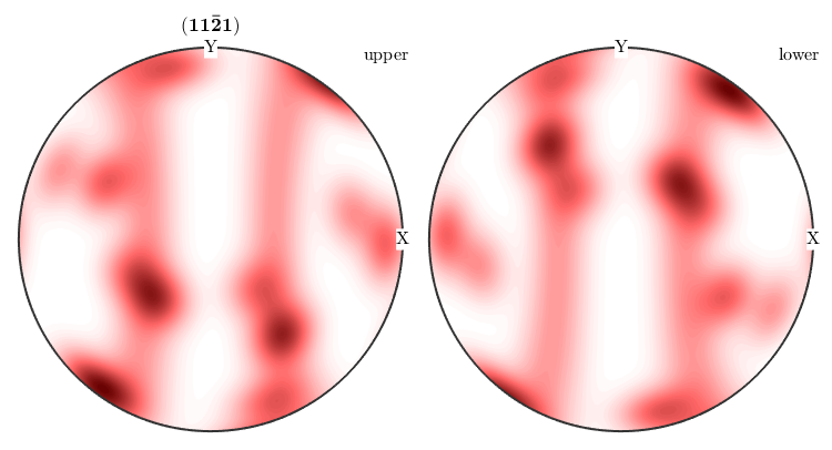
plotPDF(odf,Miller(1,1,-2,1,cs),'antipodal','complete')

Inverse Pole Figures

Plotting inverse pole figures is analogously to plotting pole figures with the only difference that you have to use the command plotIPDF and you to specify specimen directions and not crystal directions.

plotIPDF(odf,[xvector,zvector])

Imposing antipodal symmetry to the inverse pole figures halfes the fundamental region

plotIPDF(odf,[xvector,zvector],'antipodal')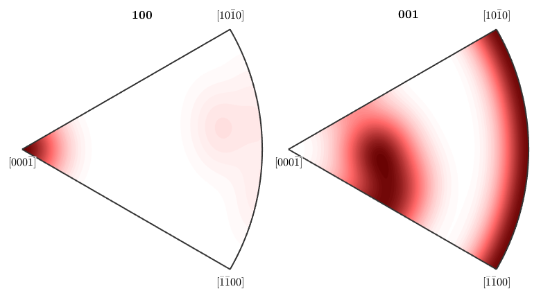

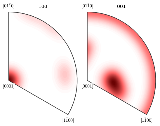
By default MTEX always plots only the fundamental region with respect to the crystal symmetry. In order to plot the complete inverse pole figure you have to use the option complete.

plotIPDF(odf,[xvector,zvector],'complete','upper')

This illustrates also more clearly the effect of the antipodal symmetry

plotIPDF(odf,[xvector,zvector],'complete','antipodal','upper')

ODF Sections

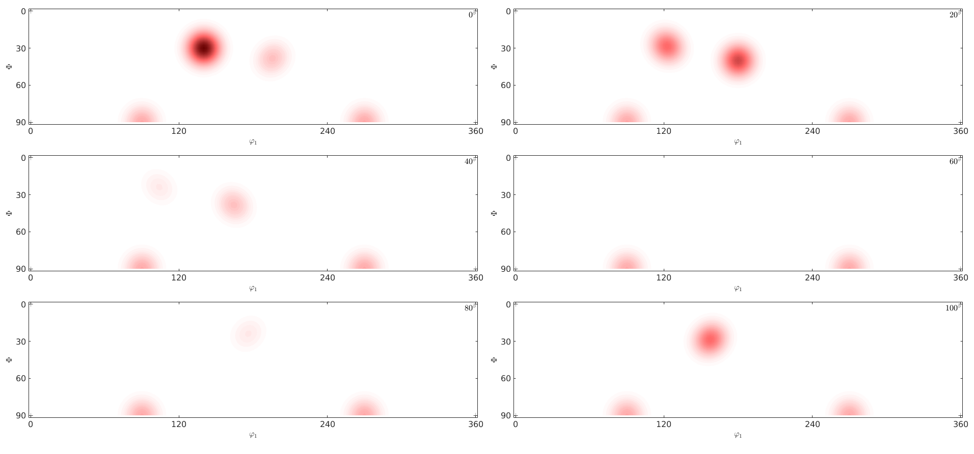
Plotting an ODF in two dimensional sections through the orientation space is done using the command plot. By default the sections are at constant angles phi2. The number of sections can be specified by the option sections

plot(odf,'sections',6,'silent')

One can also specify the phi2 angles of the sections explicitly

plot(odf,'phi2',[25 30 35 40]*degree,'contourf','silent')

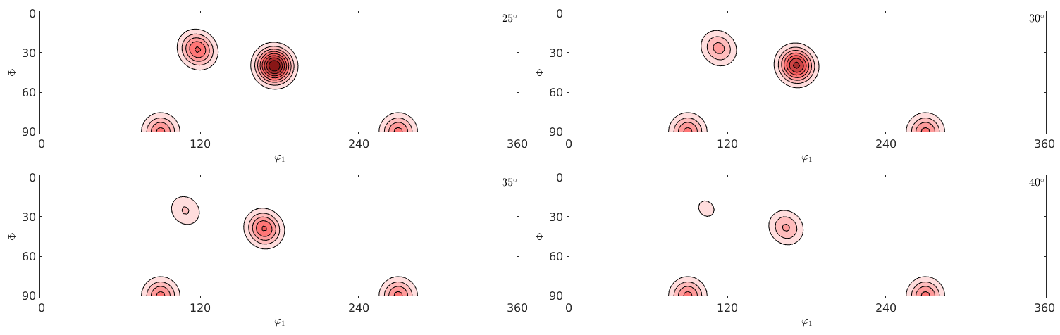
Beside the standard phi2 sections MTEX supports also sections according to all other Euler angles.

phi2 (default)
phi1
alpha (Matthies Euler angles)
gamma (Matthies Euler angles)
sigma (alpha+gamma)

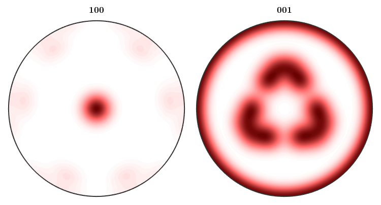
In this context the authors of MTEX recommend the sigma sections as they provide a much less distorted representation of the orientation space. They can be seen as the (001) pole figure splitted according to rotations about the (001) axis. Lets have a look at the 001 pole figure

plotPDF(odf,Miller(0,0,0,1,cs))

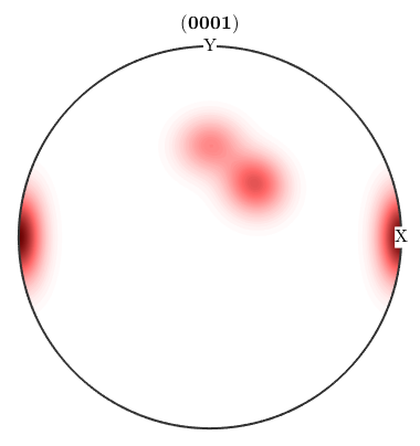
We observe three spots. Two in the center and one at 100. When splitting the pole figure, i.e. plotting the odf as sigma sections

plot(odf,'sections',6,'silent','sigma')

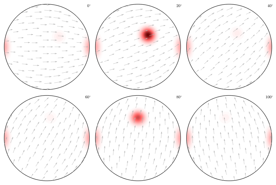
we can clearly distinguish the two spots in the middle indicating two radial symmetric portions. On the other hand the spots at 001 appear in every section indicating a fibre at position [001](100). Knowing that sigma sections are nothing else then the splitted 001 pole figure they are much more simple to interpret then usual phi2 sections.

Plotting the ODF along a fibre

For plotting the ODF along a certain fibre we have the command

close all
f = fibre(Miller(1,2,-3,2,cs),vector3d(2,1,1));
plot(odf,f,'LineWidth',2);

Fourier Coefficients

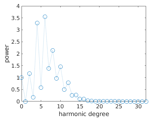
A last way to visualize an ODF is to plot its Fourier coefficients

close all;
fodf = FourierODF(odf,32)
plotFourier(fodf)

 
fodf = ODF  
  crystal symmetry : 321, X||a*, Y||b, Z||c*
  specimen symmetry: 1
 
  Harmonic portion:
    degree: 25
    weight: 1

Axis / Angle Distribution

Let us consider the uncorrelated missorientation ODF corresponding to our model ODF.

mdf = calcMDF(odf)

 
mdf = MDF  
  crystal symmetry : 321, X||a*, Y||b, Z||c*
  crystal symmetry : 321, X||a*, Y||b, Z||c*
  antipodal:         true
 
  Harmonic portion:
    degree: 23
    weight: 1

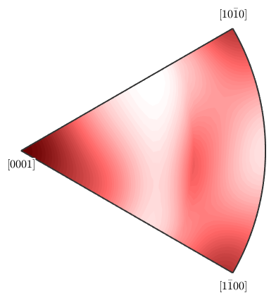
Then we can plot the distribution of the rotation axes of this missorientation ODF

plotAxisDistribution(mdf)

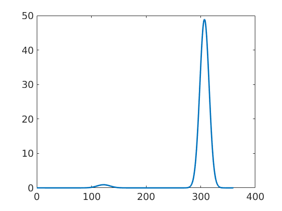
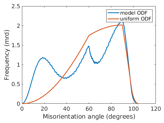
and the distribution of the missorientation angles and compare them to a uniform ODF

close all
plotAngleDistribution(mdf)
hold all
plotAngleDistribution(cs,cs)
hold off
legend('model ODF','uniform ODF')

Finally, lets set back the default colormap.

setMTEXpref('defaultColorMap',WhiteJetColorMap);