
The simulated example represents the olivine single crystal 7506 (Durham and Goetze, 1977), deformed in the [110]c orientation for which the compression direction bisects the angle between [100] and [010]. The simulated section replicates the plane strain section, i.e. in the figures below the compression direction is top to bottom in the plane of the figures. The scripts for calculation of dislocation density can be used with acquired EBSD data after denoising.
Generate text file containing EBSD data on a regular grid
% CSa defines properties of phases. By default 'notIndexed' is phase 0.
CSa = {'notIndexed',...
  crystalSymmetry('mmm', [4.756 10.207 5.98], 'mineral', 'Forsterite')};

% This makes it easier to add angular gradients.

% Set grid dimensions.
%
lx = 50;
ly = 50;
sizem = lx *ly;

% initialize matrices
[xx, yy] = meshgrid(1:lx,1:ly);
pos = vector3d(xx,yy,0);

% Set Euler angles.
% 0 180 45: replicates orientation of axes relative to angular changes in
% x and y as for 7506. z is perpendicular to the plane of the section.

% Add angular gradients to ph1
ph1 = 0.1 * (xx-yy) * degree;
rot = rotation.byEuler(ph1,180*degree,45*degree);


ebsd = EBSD(pos,rot,ones(numel(rot),1),CSa,struct);


% generate grain
segang = 10*degree; % define angle to identify grains
subang = 1*degree; % angle for sub boundaries (V5.5)

[grains,ebsd] = calcGrains(ebsd,'threshold',[subang segang],'unitCell');

% Plot orientation gradient and show crystal axes
% Color mean orientation as white and scale maximum saturation to fit the maximum misorientation angle
ipfKey = ipfHSVKey(ebsd);
ipfKey.inversePoleFigureDirection = mean(ebsd.orientations) * ipfKey.whiteCenter;
ipfKey.maxAngle = 5*degree; % adjust to magnitude of gradient

% select the grain for plotting of axes
CS = ebsd('forsterite').CS;
gsel = grains(1);
dira = gsel.meanOrientation * Miller(1,0,0,gsel.CS);
dirb = gsel.meanOrientation * Miller(0,1,0,gsel.CS);
dirc = gsel.meanOrientation * Miller(0,0,1,gsel.CS);
% lenght of plotted arrows
len = 0.1*gsel.diameter;

figure
plot(ebsd,ipfKey.orientation2color(ebsd.orientations))
hold on
ha = quiver(gsel,dira,len.*dira,'autoScale','off');
ha.Color='red'; ha.LineWidth = 1;
hb = quiver(gsel,dirb,'autoScale','off');
hb.Color='green'; hb.LineWidth = 1;
hc = quiver(gsel,dirc,'autoScale','off');
hc.Color='blue'; hc.LineWidth = 1;
hold off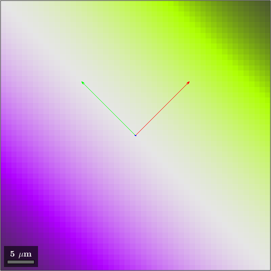
Define dislocation types for olivine with 3 orthogonal Burgers vectors
For lattices other than cubic and hexagonal MTEX takes the Burgers vector length of a screw dislocation to be the full unit cell dimension, and warns that it could not determine it automatically. For the primitive orthorhombic cell of olivine that default is the value we want - the lengths come out as a, b and c - so the warning can be ignored here.
% Define edge dislocations
sSo1 = slipSystem(Miller(1,0,0,CS,'uvw'),Miller(0,1,0,CS,'hkl'));
sSo2 = slipSystem(Miller(1,0,0,CS,'uvw'),Miller(0,0,1,CS,'hkl'));
sSo3 = slipSystem(Miller(0,0,1,CS,'uvw'),Miller(1,0,0,CS,'hkl'));
sSo4 = slipSystem(Miller(0,0,1,CS,'uvw'),Miller(0,1,0,CS,'hkl'));
sSo5 = slipSystem(Miller(0,1,0,CS,'uvw'),Miller(1,0,0,CS,'hkl'));
sSo6 = slipSystem(Miller(0,1,0,CS,'uvw'),Miller(0,0,1,CS,'hkl'));

%assemble
sSo = cat(5,sSo1,sSo2,sSo3,sSo4,sSo5,sSo6);

% to create dislocation systems need to symmetrise slip system
sSs=sSo.symmetrise('antipodal');

% Screw dislocations are generated by dislocationSystem
dSo=dislocationSystem(sSs);

% Normalized dislocation energies from Heinisch et al. Table 2
dSo.u = [0.73; 0.74; 1.0; 0.88; 2.36; 2.64; 0.65; 1.91; 0.46];

clear sSo6 sSo5 sSo4 sSo3 sSo2 sSo1 sSo sSs
% Show dislocation types and their energy. Note that Burgers vector and
% line vector directions are shown, not the glide plane. Also note order.
dSo
Warning: I could not determine the correct length of the Burgers vector.
Please adjust it manually.
Warning: I could not determine the correct length of the Burgers vector.
Please adjust it manually.
dSo = dislocationSystem
mineral: Forsterite (mmm)
edge dislocations : 6 × 1
Burgers vector line vector energy length
[1 0 0] [0 0 1] 0.73 4.76
[1 0 0] [0 -1 0] 0.74 4.76
[0 0 1] [0 1 0] 1 5.98
[0 0 1] [-1 0 0] 0.88 5.98
[0 1 0] [0 0 -1] 2.36 10.21
[0 1 0] [1 0 0] 2.64 10.21
screw dislocations: 3 × 1
Burgers vector energy length
[0 0 1] 0.65 5.98
[0 1 0] 1.91 10.21
[1 0 0] 0.46 4.76Calculate dislocation density
Acquired data needs to be denoised first!
% reshape EBSD data on a regular square grid
[ebsdG,newId] = gridify(ebsd('fo'));
% compute curvature tensors
kappa = ebsdG.curvature;
% dislocation tensor is in crystal coordinates, need to rotate it into
% specimen coordinates
dSRot = ebsdG.orientations * dSo;
% fit dislocation to curvature tensor. Dislocation density rho is 9 column
% vector. factor normalizes from acquisition step size in micron to /m2
[rho,factor] = fitDislocationSystems(kappa,dSRot);

% Calculate dislocation density for individual dislocation types
% Distributions are non-Gaussian, use median to represent each type
% rho is initiated with NaN, omit for median
dti = zeros(size(rho));
for ii = 1 : 9
  dti(:,ii) = factor * abs(rho(:,ii) .* dSRot(:,ii).u);
  dSlip(ii)=median(dti(:,ii),'omitnan');
end

% sum dislocation types to total dislocation density gnd
gnd = sum(dti,2);
% median of total dislocation density for a map
rhoAll = median(gnd,'omitnan')

% Reorder individual dislocation types for display in the sequence:
%[100](010) [100](001) [001](100) [001](010) [100]s [001]s [010](100) [010](001) [010]
rhoSlip = round([dSlip(1:4), dSlip(9), dSlip(7), dSlip(5:6), dSlip(8)],3,'significant')
rhoAll =
3.9366e+12
rhoSlip =
1.0e+12 *
Columns 1 through 7
3.7900 0.0000 0 0 0.0000 0.0000 0.1490
Columns 8 through 9
0.0000 0.0000Plot map of dislocation density
supersizeme is an optional function that scales the font sizes of all text elements in a figure. It can be downloaded from https://www.mathworks.com/matlabcentral/fileexchange/67644-supersizeme-varargin- increasing the fontsize is useful for presentations and publications
figure
% increasing the font size requires additional space around figure
newMtexFigure('outerPlotSpacing',20)
plot(ebsdG,gnd)
hold on
plot(grains.boundary,'edgecolor','k','linewidth',0.2)
plot(ebsd('notIndexed'),'FaceColor',[0.8 0.8 0.8]);
plot(grains.innerBoundary,'linewidth',0.5,'edgeColor','r');
hold off
set(gca,'ColorScale','log');
% Adjust limits of color scale to show structure
set(gca,'CLim',[1e12 1.1e14]);
mtexColorbar('title','Dislocation density, m^{-2}','fontSize',20)
legend('off')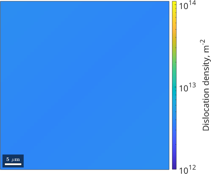
Plot dislocation densities for individual dislocation types
Order of dislocation types generated by dislocationSystem
% Dislocation type
% [100](010) [100](001) [001](100) [001](010) [100]s [001]s [010](100) [010](001) [010]s

% Corresponding column in rho
%     1          2          3         4         9      7        5        6          8

% Assign label for plotting of individual slip systems
slab = ["[100](010)","[100](001)","[001](100)","[001](010)","[010](100)","[010](001)",...
    "[001] screw","[010] screw","[100] screw"];

% set color scale for plots
mind = 5e10; maxd = 1e13;
db = 0.5; % linewidth for gb

figure
newMtexFigure('nrows',3,'ncols',3,'outerPlotSpacing',20)
nextAxis(1,1)
ind = 1;
plot(ebsdG,dti(:,ind))%,'micronbar','off')
set(gca,'ColorScale','log');
set(gca,'CLim',[mind maxd]);
hold on; plot(grains.boundary,'linewidth',db); hold off
title(slab(ind),'FontWeight','normal','fontsize',13)

nextAxis(1,2)
ind = 2;
plot(ebsdG,dti(:,ind),'micronbar','off')
set(gca,'ColorScale','log');
set(gca,'CLim',[mind maxd]);
hold on; plot(grains.boundary,'linewidth',db); hold off
title(slab(ind),'FontWeight','normal','fontsize',13)

nextAxis(2,1)
ind = 3;
plot(ebsdG,dti(:,ind),'micronbar','off')
set(gca,'ColorScale','log');
set(gca,'CLim',[mind maxd]);
hold on; plot(grains.boundary,'linewidth',db); hold off
title(slab(ind),'FontWeight','normal','fontsize',13)

nextAxis(2,2)
ind = 4;
plot(ebsdG,dti(:,ind),'micronbar','off')
set(gca,'ColorScale','log');
set(gca,'CLim',[mind maxd]);
hold on; plot(grains.boundary,'linewidth',db); hold off
title(slab(ind),'FontWeight','normal','fontsize',13)

nextAxis(1,3)
ind = 9;
plot(ebsdG,dti(:,ind),'micronbar','off')
set(gca,'ColorScale','log');
set(gca,'CLim',[mind maxd]);
hold on; plot(grains.boundary,'linewidth',db); hold off
title(slab(ind),'FontWeight','normal','fontsize',13)

nextAxis(2,3)
ind = 7;
plot(ebsdG,dti(:,ind),'micronbar','off')
set(gca,'ColorScale','log');
set(gca,'CLim',[mind maxd]);
hold on; plot(grains.boundary,'linewidth',db); hold off
title(slab(ind),'FontWeight','normal','fontsize',13)

nextAxis(3,1)
ind = 5;
plot(ebsdG,dti(:,ind),'micronbar','off')
set(gca,'ColorScale','log');
set(gca,'CLim',[mind maxd]);
hold on; plot(grains.boundary,'linewidth',db); hold off
title(slab(ind),'FontWeight','normal','fontsize',13)
nextAxis(3,2)
ind = 6;
plot(ebsdG,dti(:,ind),'micronbar','off')
set(gca,'ColorScale','log');
set(gca,'CLim',[mind maxd]);
hold on; plot(grains.boundary,'linewidth',db); hold off
title(slab(ind),'FontWeight','normal','fontsize',13)

nextAxis(3,3)
ind = 8;
plot(ebsdG,dti(:,ind),'micronbar','off')
set(gca,'ColorScale','log');
set(gca,'CLim',[mind maxd]);
hold on; plot(grains.boundary,'linewidth',db); hold off
title(slab(ind),'FontWeight','normal','fontsize',13)
mtexColorbar('title','Dislocation density, m^{-2}','fontSize',20)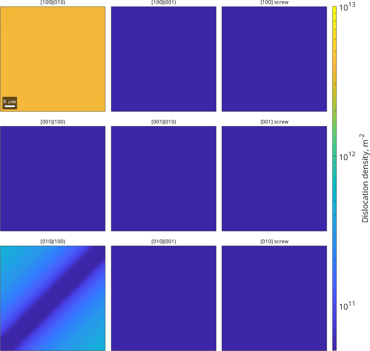
References
Durham, WB, C. Goetze, Plastic flow of oriented single crystals of olivine, Journal of Geophysical Research, 82, 5737 - 5753, 1977
Faul, U. Dislocation structure of deformed olivine single crystals from conventional EBSD maps, Physics and Chemistry of Minerals, 48, 2021, https://doi.org/10.1007/s00269-021-01157-3
Citing this page.
This page is part of the documentation of
MTEX, a free and open
source MATLAB toolbox for analyzing and modeling crystallographic textures.
It was written by The MTEX Developers and is published at
https://mtex-toolbox.github.io/SynEBSD.html.
If you use MTEX, or reuse text or figures from this page, in your research,
please cite
F. Bachmann, R. Hielscher, H. Schaeben: Texture Analysis with MTEX - Free and Open Source Software Toolbox, Solid State Phenomena 160 (2010), 63-68. 10.4028/www.scientific.net/SSP.160.63
BibTeX
@article{bachmann2010mtex,
  author  = {F. Bachmann and R. Hielscher and H. Schaeben},
  title   = {Texture Analysis with MTEX - Free and Open Source Software Toolbox},
  journal = {Solid State Phenomena},
  volume  = {160},
  pages   = {63-68},
  year    = {2010},
  doi     = {10.4028/www.scientific.net/SSP.160.63},
  url     = {https://doi.org/10.4028/www.scientific.net/SSP.160.63}
}
Other papers describing specific MTEX methods are listed under Publications — please cite the one that best fits your application. The MTEX source code is licensed under the GNU General Public License v2.0; the text and figures of this documentation are licensed under CC BY 4.0, which permits reuse — including by automated systems — provided The MTEX Developers and this page are credited.