MTEX - Analysing Neutron Pole Figures (Dubna)

Detailed demonstration of the MTEX toolbox at the Dubna data example.

The data where meassured by Florian Wobbe at Dubna 2005 of a Quarz specimen using Neutron diffraction.

Import diffraction data

% specify scrystal and specimen symmetry
cs = crystalSymmetry('-3m',[1.4,1.4,1.5]);

% specify file names
fname = {...
  fullfile(mtexDataPath,'PoleFigure','dubna', 'Q(10-10)_amp.cnv'),...
  fullfile(mtexDataPath,'PoleFigure','dubna','Q(10-11)(01-11)_amp.cnv'),...
  fullfile(mtexDataPath,'PoleFigure','dubna','Q(11-22)_amp.cnv')};

% specify crystal directions
h = {Miller(1,0,-1,0,cs),[Miller(0,1,-1,1,cs),Miller(1,0,-1,1,cs)],Miller(1,1,-2,2,cs)};

% specify structure coefficients
c = {1,[0.52 ,1.23],1};

% import pole figure data
pf = PoleFigure.load(fname,h,cs,'superposition',c)

 
pf = PoleFigure  
  crystal symmetry : -3m1, X||a*, Y||b, Z||c*
  specimen symmetry: 1
 
  h = (10-10), r = 72 x 19 points
  h = (01-11)(10-11), r = 72 x 19 points
  h = (11-22), r = 72 x 19 points

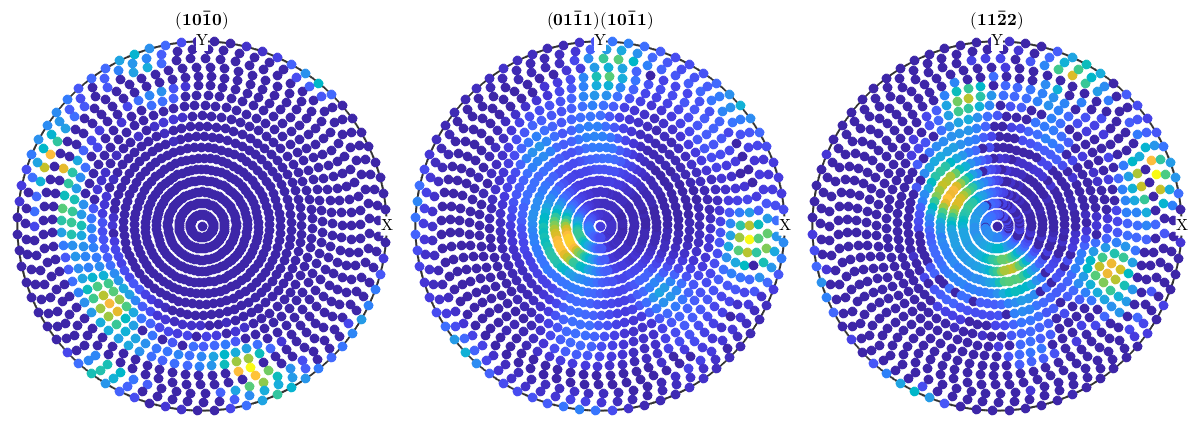
plot pole figures

plot(pf)

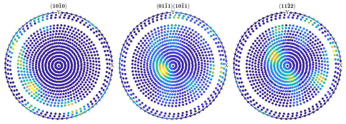
Correct pole figures

pf_corrected = pf(pf.r.theta < 70*degree | pf.r.theta > 75*degree);

plot(pf_corrected)

Rotate pole figures

pf_rotated = rotate(pf_corrected,axis2quat(xvector,45*degree));
plot(pf_rotated,'antipodal')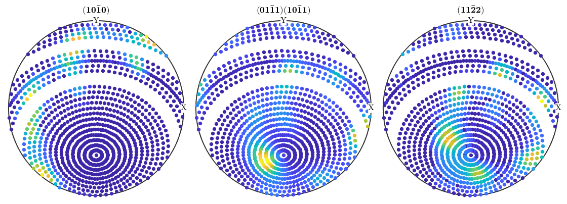

Recalculate ODF

We use here the option 'background' to specify the approximative background radiation and to increase the accuracy of the reconstruction. Furthermore, we have seen from the pole figures that the ODF is quit sharp and hence using the zero range method reduces the computational time.

odf = calcODF(pf_corrected,'background',10,'zero_range')

 
odf = ODF  
  crystal symmetry : -3m1, X||a*, Y||b, Z||c*
  specimen symmetry: 1
 
  Radially symmetric portion:
    kernel: de la Vallee Poussin, halfwidth 10°
    center: 19777 orientations, resolution: 5°
    weight: 1

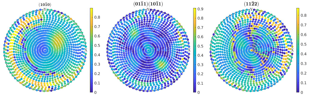
Error analysis

% calc RP1 error
calcError(pf_corrected,odf,'RP',1)

% difference plot
plotDiff(pf,odf)

mtexColorbar

progress: 100%
ans =
    0.6324    0.3336    0.4106
progress: 100%

Recalculate c-axis pole figures

plotPDF(odf,Miller(0,0,1,cs),'antipodal')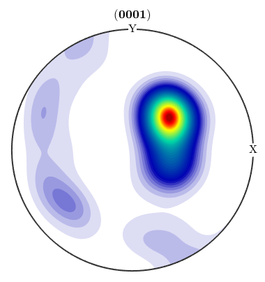

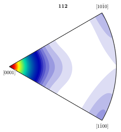
Plot inverse pole figure

plotIPDF(odf,vector3d(1,1,2))

plot recalculated ODF

plot(odf,'sections',6,'silent','sigma')

progress: 100%

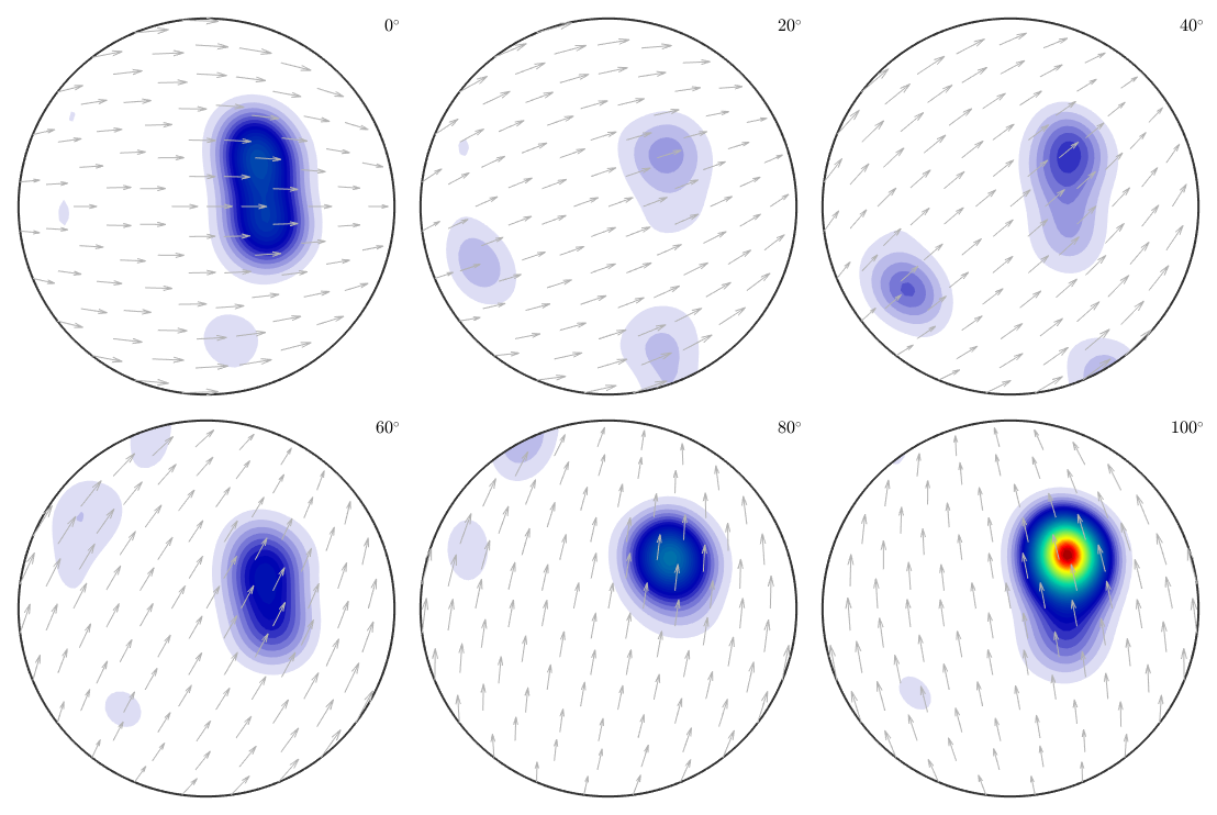
rotate ODF back

odfrotated = rotate(odf,axis2quat(xvector,45*degree));
plot(odfrotated,'sections',8,'sigma');
annotate(calcModes(odfrotated),'marker','o',...
  'MarkerFaceColor','none','MarkerEdgeColor','k');

progress: 100%
progress: 100%

volume analysis

volume(odf,calcModes(odf),20*degree)

progress: 100%
ans =
    0.2617