Twinning Analysis

Data import and grain detection

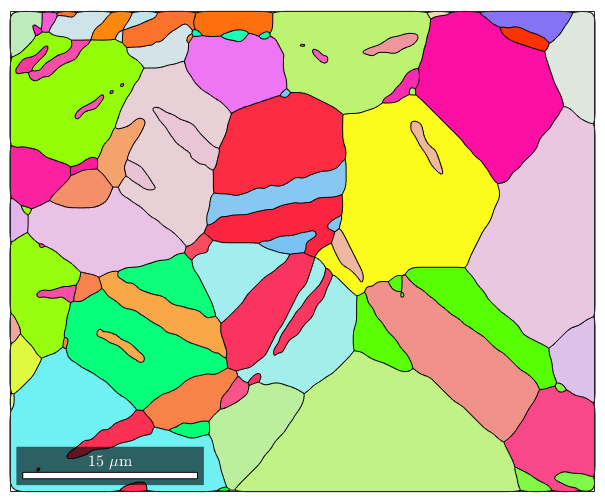
Lets import some Magnesium data that are full of grains and segment grain within the data set.

% load some example data
mtexdata twins

% segment grains
[grains,ebsd.grainId,ebsd.mis2mean] = calcGrains(ebsd('indexed'),'angle',5*degree);

% remove two pixel grains
ebsd(grains(grains.grainSize<=2)) = [];
[grains,ebsd.grainId,ebsd.mis2mean] = calcGrains(ebsd('indexed'),'angle',5*degree);

% smooth them
grains = grains.smooth(5);

% visualize the grains
plot(grains,grains.meanOrientation)

% store crystal symmetry of Magnesium
CS = grains.CS;

  I'm going to colorize the orientation data with the 
  standard MTEX colorkey. To view the colorkey do:
 
  colorKey = ipfColorKey(ori_variable_name)
  plot(colorKey)

Now we can extract from the grains its boundary and save it to a separate variable

gB = grains.boundary

 
gB = grainBoundary  
 
 Segments   mineral 1  mineral 2
      600  notIndexed  Magnesium
     3164   Magnesium  Magnesium

The output tells us that we have 3219 Magnesium to Magnesium boundary segments and 606 boundary segements where the grains are cut by the scanning boundary. To restrict the grain boundaries to a specific phase transistion you shall do

gB_MgMg = gB('Magnesium','Magnesium')

 
gB_MgMg = grainBoundary  
 
 Segments  mineral 1  mineral 2
     3164  Magnesium  Magnesium

Back to Top

Properties of grain boundaries

A variable of type grain boundary contains the following properties

These can be used to colorize the grain boundaries. By the following command, we plot the grain boundaries colorized by the misorientation angle

plot(gB_MgMg,gB_MgMg.misorientation.angle./degree,'linewidth',2)
mtexColorbar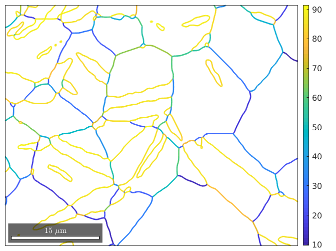

We observe many grain boundaries with a large misorientation angle of about 86 degrees. Those grain boundaries are most likely twin boundaries. To detect them more precisely we define first the twinning as a misorientation, which is reported in literature by (1,1,-2,0) parallel to (2,-1,-1,0) and (-1,0,1,1) parallel to (1,0,-1,1). In MTEX it is defined by

twinning = orientation.map(Miller(1,1,-2,0,CS),Miller(2,-1,-1,0,CS),...
  Miller(-1,0,1,1,CS),Miller(-1,1,0,1,CS))

 
twinning = misorientation  
  size: 1 x 1
  crystal symmetry : Magnesium (6/mmm, X||a*, Y||b, Z||c*)
  crystal symmetry : Magnesium (6/mmm, X||a*, Y||b, Z||c*)
 
  Bunge Euler angles in degree
  phi1  Phi phi2 Inv.
   300    0    0    0
 

The followin lines show that the twinning is actually a rotation about axis (-2110) and angle 86.3 degree

% the rotational axis
round(twinning.axis)

% the rotational angle
twinning.angle / degree

 
ans = Miller  
 size: 1 x 1
 mineral: Magnesium (622, X||a*, Y||b, Z||c*)
  h  1
  k  0
  i -1
  l  0
ans =
     0

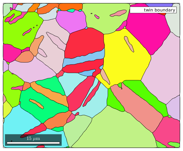
Next, we check for each boundary segment whether it is a twinning boundary, i.e., whether boundary misorientation is close to the twinning.

% restrict to twinnings with threshold 5 degree
isTwinning = angle(gB_MgMg.misorientation,twinning) < 5*degree;
twinBoundary = gB_MgMg(isTwinning)

% plot the twinning boundaries
plot(grains,grains.meanOrientation)
%plot(ebsd('indexed'),ebsd('indexed').orientations)
hold on
%plot(gB_MgMg,angle(gB_MgMg.misorientation,twinning),'linewidth',4)
plot(twinBoundary,'linecolor','w','linewidth',2,'displayName','twin boundary')
hold off

 
twinBoundary = grainBoundary  
  grain boundary is empty!
  I'm going to colorize the orientation data with the 
  standard MTEX colorkey. To view the colorkey do:
 
  colorKey = ipfColorKey(ori_variable_name)
  plot(colorKey)

Back to Top

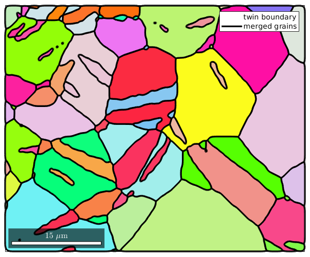
Merge twins along twin boundaries

Grains that have a common twin boundary are assumed to inherite from one common grain. To reconstruct those initial grains we merge grains together which have a common twin boundary. This is done by the command merge.

[mergedGrains,parentId] = merge(grains,twinBoundary);

% plot the merged grains
%plot(ebsd,ebsd.orientations)
hold on
plot(mergedGrains.boundary,'linecolor','k','linewidth',2.5,'linestyle','-',...
  'displayName','merged grains')
hold off

Back to Top

Grain relationships

The second output argument paraentId of merge is a list with the same size as grains which indicates for each grain into which common grain it has been merged. The id of the common grain is usually different from the ids of the merged grains and can be found by

mergedGrains(16).id

ans =
    16

Hence, we can find all childs of grain 16 by

childs = grains(parentId == mergedGrains(16).id)

 
childs = grain2d  
 
 Phase  Grains  Pixels    Mineral  Symmetry  Crystal reference frame
     1       1    1427  Magnesium     6/mmm       X||a*, Y||b, Z||c*
 
 boundary segments: 286
 triple points: 9
 
 Id   Phase   Pixels       GOS   phi1   Phi   phi2
 16       1     1427   0.01101      4    81    195
 

Back to Top

Calculate the twinned area

We can also answer the question about the relative area of these initial grains that have undergone twinning to total area.

twinId = unique(gB_MgMg(isTwinning).grainId);

% compute the area fraction
sum(area(grains(twinId))) / sum(area(grains)) * 100

ans =
     0

Back to Top

Setting Up the EBSD Data for the Merged Grains

Note that the Id's of the merged grains does not fit the grainIds stored in the initial ebsd variable. As a consequence, the following command will not give the right result

plot(mergedGrains(16).boundary,'linewidth',2)
hold on
plot(ebsd(mergedGrains(16)),ebsd(mergedGrains(16)).orientations)
hold off

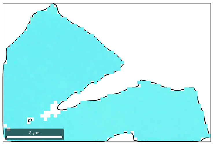
In order to update the grainId in the ebsd variable to the merged grains, we proceed as follows.

% copy ebsd data into a new variable to not change the old data
ebsd_merged = ebsd;

% update the grainIds to the parentIds
ebsd_merged('indexed').grainId = parentId(ebsd('indexed').grainId)

 
ebsd_merged = EBSD  
 
 Phase  Orientations     Mineral       Color  Symmetry  Crystal reference frame
     0     46 (0.2%)  notIndexed                                               
     1  22794 (100%)   Magnesium  light blue     6/mmm       X||a*, Y||b, Z||c*
 
 Properties: bands, bc, bs, error, mad, x, y, grainId, mis2mean
 Scan unit : um
 

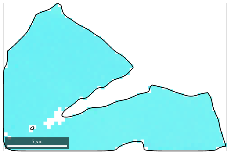
Now the variable ebsd_merged can be indexed by the merged grains, i.e.

plot(ebsd_merged(mergedGrains(16)),ebsd_merged(mergedGrains(16)).orientations)
hold on
plot(mergedGrains(16).boundary,'linewidth',2)
hold off

Back to Top

DocHelp 0.1 beta