Tensor Arithmetics
how to calculate with tensors in MTEX
MTEX offers some basic functionality to calculate with tensors as they occur in material sciense. It allows defining tensors of arbitrary rank, e.g., stress, strain, elasticity or piezoelectric tensors, to visualize them and to perform various transformations.
| On this page ... |
| Defining a Tensor |
| Importing a Tensor from a File |
| Visualization |
| Rotating a Tensor |
| The Inverse Tensor |
| Tensor Products |
Defining a Tensor
A tensor is defined by its entries and a crystal symmetry. Let us consider a simple example. First, we define some crystal symmetry
cs = crystalSymmetry('1');Next, we define a two rank tensor by its matrix
M = [[10 3 0];[3 1 0];[0 0 1]];
T = tensor(M,cs)
T = tensor
  rank   : 2 (3 x 3)
  mineral: 1, X||a, Y||b*, Z||c*

 10  3  0
  3  1  0
  0  0  1
In case the two rank tensor is diagonal the syntax simplifies to
T = tensor(diag([10 3 1]),cs)
T = tensor
  rank   : 2 (3 x 3)
  mineral: 1, X||a, Y||b*, Z||c*

 10  0  0
  0  3  0
  0  0  1
Importing a Tensor from a File
Especially for higher order tensors, it is more convenient to import the tensor entries from a file. As an example, we load the following elastic stiffness tensor
fname = fullfile(mtexDataPath,'tensor','Olivine1997PC.GPa');

cs = crystalSymmetry('mmm',[4.7646 10.2296 5.9942],'mineral','olivine');

C = stiffnessTensor.load(fname,cs)
C = stiffnessTensor
  unit   : GPa
  rank   : 4 (3 x 3 x 3 x 3)
  mineral: olivine (mmm)

  tensor in Voigt matrix representation:
 320.5  68.2  71.6     0     0     0
  68.2 196.5  76.8     0     0     0
  71.6  76.8 233.5     0     0     0
     0     0     0    64     0     0
     0     0     0     0    77     0
     0     0     0     0     0  78.7
Visualization
The default plot for each tensor is its directional magnitude, i.e. for each direction x it is plotted Q(x) = T_ijkl x_i x_j x_k x_l
setMTEXpref('defaultColorMap',blue2redColorMap);
plot(C,'complete','upper')
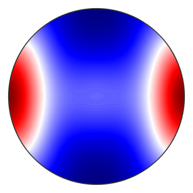
There are more specialized visualization possibilities for specific tensors, e.g., for the elasticity tensor. See section Elasticity Tensor.
Rotating a Tensor
Rotation a tensor is done by the command rotate. Let's define a rotation
r = rotation.byEuler(45*degree,0*degree,0*degree)
r = rotation
  size: 1 x 1

  Bunge Euler angles in degree
  phi1  Phi phi2 Inv.
    45    0    0    0
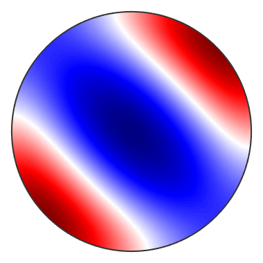
Then the rotated tensor is given by
Trot = rotate(T,r)
plot(Trot)
Trot = tensor
  rank   : 2 (3 x 3)
  mineral: 1, X||a, Y||b*, Z||c*

 6.5 3.5   0
 3.5 6.5   0
   0   0   1
Here is another example from Nye (Physical Properties of Crystals, p.120-121) for a third-rank tensor
P = [ 0 0 0 .17 0   0;
      0 0 0 0   .17 0;
      0 0 0 0   0   5.17]*10^-11;

T = tensor(P,'rank',3,'propertyname','piezoelectric modulus')

r = rotation.byAxisAngle(zvector,-45*degree);
T = rotate(T,r)
T = tensor
  propertyname: piezoelectric modulus
  rank        : 3 (3 x 3 x 3)

  tensor in compact matrix form: *10^-12
    0    0    0  1.7    0    0
    0    0    0    0  1.7    0
    0    0    0    0    0 51.7

T = tensor
  propertyname: piezoelectric modulus
  rank        : 3 (3 x 3 x 3)

  tensor in compact matrix form: *10^-12
     0     0     0     0   1.7     0
     0     0     0  -1.7     0     0
  51.7 -51.7     0     0     0     0
The Inverse Tensor
The inverse of a 2 rank tensor or a 4 rank elasticity tensor is computed by the command inv
S = inv(C)
S = complianceTensor
  unit            : 1/GPa
  rank            : 4 (3 x 3 x 3 x 3)
  doubleConvention: true
  mineral         : olivine (mmm)

  tensor in Voigt matrix representation: *10^-4
  34.85  -9.08   -7.7      0      0      0
  -9.08  60.76  -17.2      0      0      0
   -7.7  -17.2  50.85      0      0      0
      0      0      0 156.25      0      0
      0      0      0      0 129.87      0
      0      0      0      0      0 127.06
Tensor Products
In MTEX tensor products are specifies according to Einsteins summation convention, i.e. a tensor product of the form T_ij = E_ijkl S_kl has to be interpreted as a sum over the indices k and l. In MTEX this sum can be computed using the command EinsteinSum
S = EinsteinSum(C,[-1 -2 1 2],T,[-1 -2])
S = tensor
  size   : 3 x 1
  rank   : 2 (3 x 3)
  mineral: olivine (mmm)
here the negative numbers indicate the indices which are summed up. Each pair of equal negative numbers corresponds to one sum. The positive numbers indicate the order of the dimensions of the resulting tensor.
Let us consider the second example. The linear compressibility in a certain direction v of a specimen can be computed from it mean elasticity tensor E by the formula, c = S_ijkk v_i v_j where S is the compliance, i.e. the inverse of the elasticity tensor
v = xvector;
c = EinsteinSum(C,[-1 -2 -3 -3],v,-1,v,-2)
c =
  460.2500
set back the default color map.
setMTEXpref('defaultColorMap',WhiteJetColorMap)
| DocHelp 0.1 beta |