Taylor Model
% display pole figure plots with RD on top and ND west
plotx2north

% store old annotation style
storepfA = getMTEXpref('pfAnnotations');

% set new annotation style to display RD and ND
pfAnnotations = @(varargin) text(-[vector3d.X,vector3d.Y],{'RD','ND'},...
  'BackgroundColor','w','tag','axesLabels',varargin{:});

setMTEXpref('pfAnnotations',pfAnnotations);
Set up
consider cubic crystal symmetry
cs = crystalSymmetry('432');

% define a family of slip systems
sS = slipSystem.bcc(cs);

% some plane strain
q = 0;
epsilon = strainTensor(diag([1 -q -(1-q)]))

% define a crystal orientation
ori = orientation.byEuler(0,30*degree,15*degree,cs)

% compute the Taylor factor
[M,b,W] = calcTaylor(inv(ori)*epsilon,sS.symmetrise);
epsilon = strainTensor
  rank: 2 (3 x 3)

  1  0  0
  0  0  0
  0  0 -1

ori = orientation
  size: 1 x 1
  crystal symmetry : 432
  specimen symmetry: 1

  Bunge Euler angles in degree
  phi1  Phi phi2 Inv.
     0   30   15    0
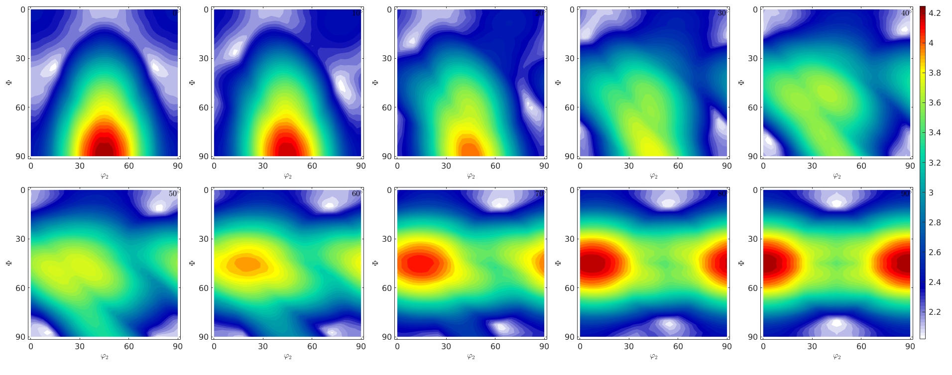
The orientation dependence of the Taylor factor
The following code reproduces Fig. 5 of the paper of Bunge, H. J. (1970). Some applications of the Taylor theory of polycrystal plasticity. Kristall Und Technik, 5(1), 145-175. http://doi.org/10.1002/crat.19700050112
% set up an phi1 section plot
sP = phi1Sections(cs,specimenSymmetry('222'));
sP.phi1 = (0:10:90)*degree;

% generate an orientations grid
oriGrid = sP.makeGrid('resolution',2.5*degree);
oriGrid.SS = specimenSymmetry;

% compute Taylor factor for all orientations
tic
[M,~,W] = calcTaylor(inv(oriGrid)*epsilon,sS.symmetrise);
toc

% plot the taylor factor
sP.plot(M,'smooth')

mtexColorbar
 computing Taylor factor: 100%
Elapsed time is 15.844487 seconds.
The orientation dependence of the spin
Compare Fig. 8 of the above paper
sP.plot(W.angle./degree,'smooth')
mtexColorbar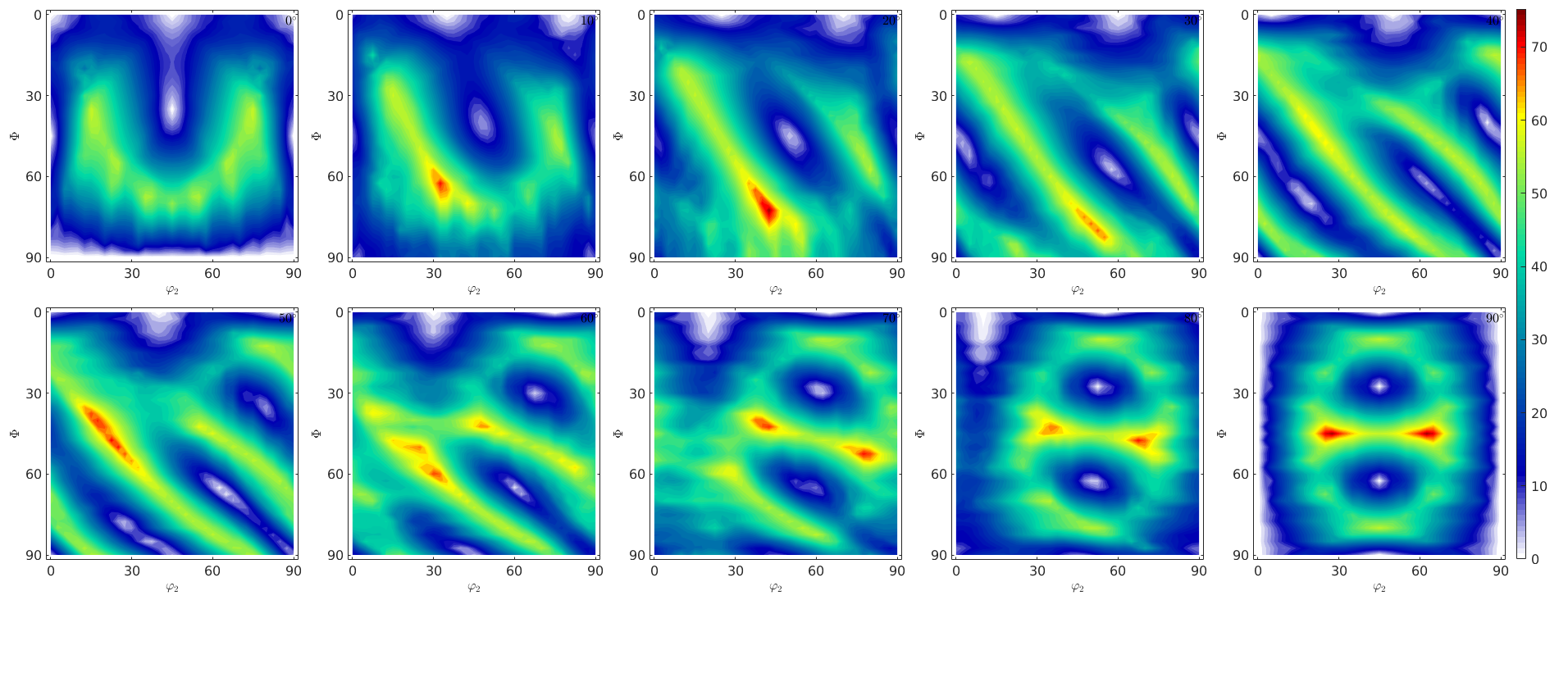
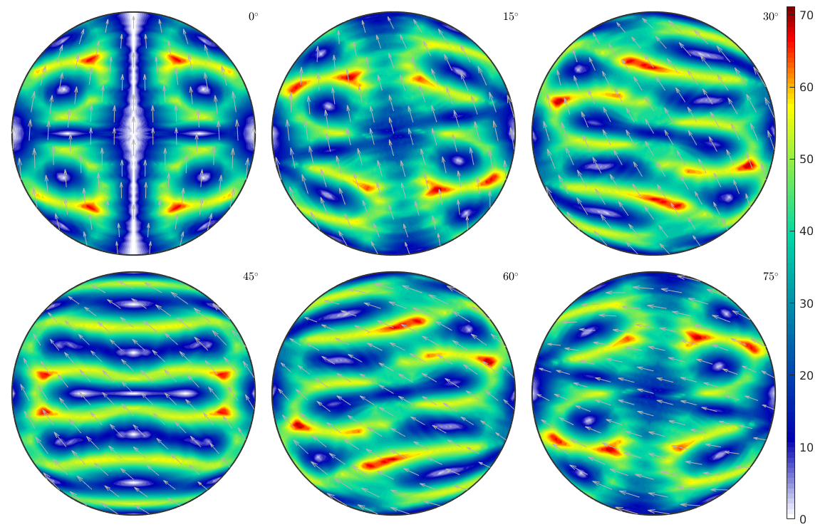
Display the crystallographic spin in sigma sections
sP = sigmaSections(cs,specimenSymmetry);
oriGrid = sP.makeGrid('resolution',2.5*degree);
[M,~,W] = calcTaylor(inv(oriGrid)*epsilon,sS.symmetrise);
sP.plot(W.angle./degree,'smooth')
mtexColorbar
computing Taylor factor: 100%
Most active slip direction
Next we consider a real world data set.
mtexdata csl

% compute grains
grains = calcGrains(ebsd('indexed'));
grains = smooth(grains,5);

% remove small grains
grains(grains.grainSize <= 2) = []
grains = grain2d

 Phase  Grains  Pixels  Mineral  Symmetry  Crystal reference frame
    -1     527  153693     iron      m-3m

 boundary segments: 21937
 triple points: 1451

 Properties: GOS, meanRotation
Next we apply the Taylor model to each grain of our data set
% some strain
q = 0;
epsilon = strainTensor(diag([1 -q -(1-q)]))

% consider fcc slip systems
sS = symmetrise(slipSystem.fcc(grains.CS));

% apply Taylor model
[M,b,W] = calcTaylor(inv(grains.meanOrientation)*epsilon,sS);
epsilon = strainTensor
  rank: 2 (3 x 3)

  1  0  0
  0  0  0
  0  0 -1
 computing Taylor factor: 100%
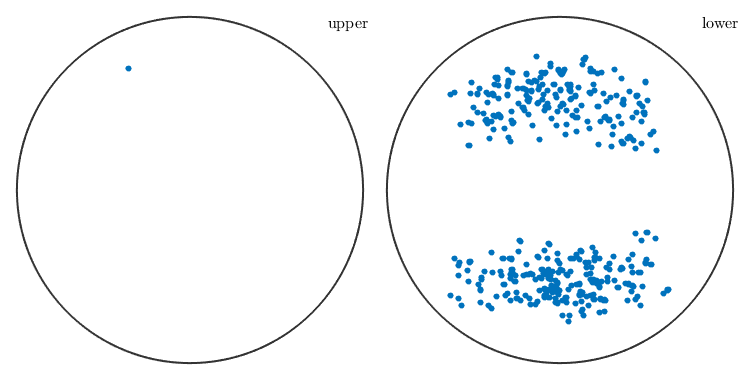
% colorize grains according to Taylor factor
plot(grains,M)
mtexColorMap white2black
mtexColorbar

% index of the most active slip system - largest b
[~,bMaxId] = max(b,[],2);

% rotate the moste active slip system in specimen coordinates
sSGrains = grains.meanOrientation .* sS(bMaxId);

% visualize slip direction and slip plane for each grain
hold on
quiver(grains,sSGrains.b,'autoScaleFactor',0.5,'displayName','Burgers vector')
hold on
quiver(grains,sSGrains.trace,'autoScaleFactor',0.5,'displayName','slip plane trace')
hold off
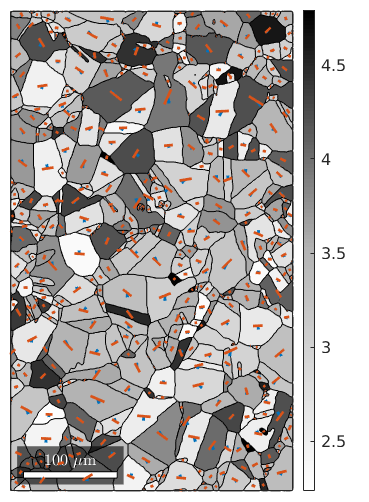
plot the most active slip directions observe that they point all towards the lower hemisphere - why? they do change if q is changed
figure(2)
plot(sSGrains.b)
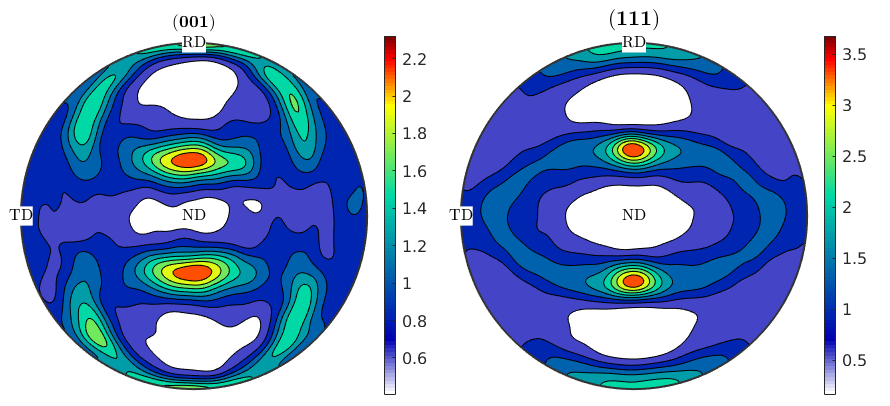
Texture evolution during rolling
% define some random orientations
ori = orientation.rand(10000,cs);

% 30 percent plane strain
q = 0;
epsilon = 0.3 * strainTensor(diag([1 -q -(1-q)]));

%
numIter = 10;
progress(0,numIter);
for sas=1:numIter

  % compute the Taylor factors and the orientation gradients
  [M,~,W] = calcTaylor(inv(ori) * epsilon ./ numIter, sS.symmetrise,'silent');

  % rotate the individual orientations
  ori = ori .* orientation(-W);
  progress(sas,numIter);
end
progress: 100%
% plot the resulting pole figures

% set new annotation style to display RD and ND
pfAnnotations = @(varargin) text([vector3d.X,vector3d.Y,vector3d.Z],{'RD','TD','ND'},...
  'BackgroundColor','w','tag','axesLabels',varargin{:});
setMTEXpref('pfAnnotations',pfAnnotations);

plotPDF(ori,Miller({0,0,1},{1,1,1},cs),'contourf')
mtexColorbar
restore MTEX preferences
setMTEXpref('pfAnnotations',storepfA);
Inverse Taylor
Use with care!
oS = axisAngleSections(cs,cs,'antipodal');
oS.angles = 10*degree;

ori = oS.makeGrid;

[M,b,eps] = calcInvTaylor(ori,sS.symmetrise);
computing Taylor factor: 100%
plot(oS,M,'contourf')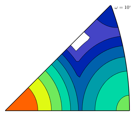
| DocHelp 0.1 beta |