Specimen Directions
How to represent directions with respect to the sample or specimen reference system.
| On this page ... |
| Cartesian Coordinates |
| Polar Coordinates |
| Calculating with Specimen Directions |
| Lists of vectors |
| Indexing lists of vectors |
Specimen directions are three dimensional vectors in the Euclidean space represented by coordinates with respect to an external specimen coordinate system X, Y, Z. In MTEX, specimen directions are represented by variables of the class vector3d.
Cartesian Coordinates
The standard way to define specimen directions is by its coordinates.
v = vector3d(1,2,3)
v = vector3d
 size: 1 x 1
  x y z
  1 2 3
This gives a single vector with coordinates (1,1,0) with respect to the X, Y, Z coordinate system. Lets visualize this vector
plot(v)
annotate([vector3d.X,vector3d.Y,vector3d.Z],'label',{'X','Y','Z'},'backgroundcolor','w')
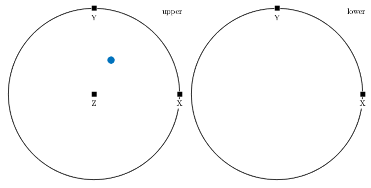
Note that the alignment of the X, Y, Z axes is only a plotting convention, which can be easily changed without changing the coordinates, e.g., by setting
plotx2north
plot(v,'grid')
annotate([vector3d.X,vector3d.Y,vector3d.Z],'label',{'X','Y','Z'},'backgroundcolor','w')
One can easily access the coordinates of any vector by
v.x
ans =
     1
or change it by
v.x = 0
v = vector3d
 size: 1 x 1
  x y z
  0 2 3
Polar Coordinates
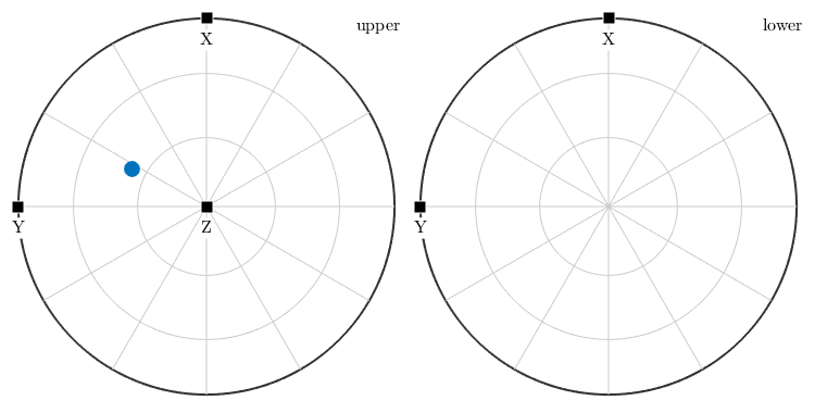
A second way to define specimen directions is by polar coordinates, i.e. by its polar angle and its azimuth angle. This is done by the option polar.
polar_angle = 60*degree;
azimuth_angle = 45*degree;
v = vector3d.byPolar(polar_angle,azimuth_angle)

plotx2east
plot(v,'grid')
annotate([vector3d.X,vector3d.Y,vector3d.Z],'label',{'X','Y','Z'},'backgroundcolor','w')
v = vector3d
 size: 1 x 1
         x        y        z
  0.612372 0.612372      0.5
Analogously as for the Cartesian coordinates we can access and change polar coordinates directly by
v.rho ./ degree   % the azimuth angle in degree
v.theta ./ degree % the polar angle in degree
ans =
   45.0000
ans =
   60.0000
Calculating with Specimen Directions
In MTEX, one can calculate with specimen directions as with ordinary numbers, i.e. we can use the predefined vectors xvector, yvector, and zvector and set
v = xvector + 2*yvector
v = vector3d
 size: 1 x 1
  x y z
  1 2 0
Moreover, all basic vector operations as "+", "-", "*", inner product, product are implemented in MTEX.
u = dot(v,xvector) * yvector + 2 * cross(v,zvector)
u = vector3d
 size: 1 x 1
  x  y  z
  4 -1  0
Beside the standard linear algebra operations there are also the following functions available in MTEX.
angle(v1,v2) % angle between two specimen  directions
dot(v1,v2)   % inner product
cross(v1,v2) % cross product
norm(v)      % length of the specimen directions
sum(v)       % sum over all specimen directions in v
mean(v)      % mean over all specimen directions in v
polar(v)     % conversion to spherical coordinates
A simple example to apply the norm function is to normalize specimen directions
v ./ norm(v)
ans = vector3d
 size: 1 x 1
         x        y        z
  0.447214 0.894427        0
Lists of vectors
As any other MTEX variable you can combine several vectors to a list of vectors and all bevor mentioned operators operations will work elementwise on a list of vectors. See < WorkinWithLists.html Working with lists> on how to manipulate lists in Matlab.
Large lists of vectors can be imported from a text file by the command
fname = fullfile(mtexDataPath,'vector3d','vectors.txt');
v = vector3d.load(fname,'ColumnNames',{'polar angle','azimuth angle'})
v = vector3d
 size: 1000 x 1
and exported by the command
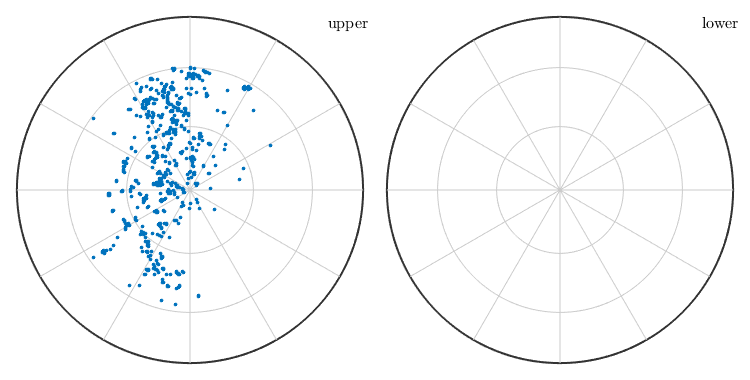
export(v,fname,'polar')In order to visualize large lists of specimen directions scatter plots
scatter(v,'upper')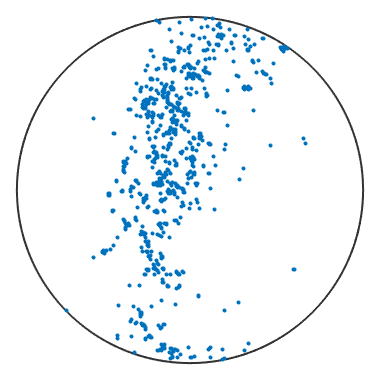
or contour plots may be helpful
contourf(v,'upper')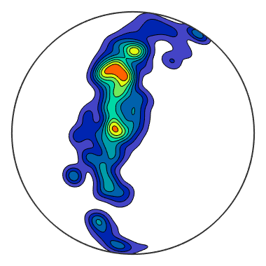
Indexing lists of vectors
A list of vectors can be indexed directly by specifying the ids of the vectors one is interested in, e.g.
v([1:5])
ans = vector3d
 size: 5 x 1
           x          y          z
    0.174067   0.983688  0.0453682
  0.00905843   0.821965   0.569466
    0.430105   0.900869  0.0586948
   -0.447234  0.0186977   0.894221
   -0.139746   0.555614   0.819612
gives the first 5 vectors from the list, or by logical indexing. The following command plots all vectors with an polar angle smaller then 60 degree
scatter(v(v.theta<60*degree),'grid','on')
| DocHelp 0.1 beta |