The SantaFe example
Simulate a set of pole figures for the SantaFe standard ODF, estimate an ODF and compare it to the inital SantaFe ODF.
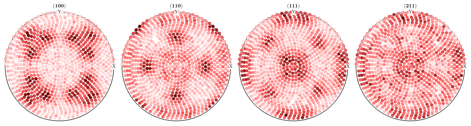
Simulate pole figures
CS = crystalSymmetry('m-3m');

% crystal directions
h = [Miller(1,0,0,CS),Miller(1,1,0,CS),Miller(1,1,1,CS),Miller(2,1,1,CS)];

% specimen directions
r = equispacedS2Grid('resolution',5*degree,'antipodal');

% pole figures
pf = calcPoleFigure(SantaFe,h,r);

% add some noise
pf = noisepf(pf,100);

% plot them
plot(pf,'MarkerSize',5)
mtexColorMap LaboTeX
ODF Estimation with Ghost Correction
rec = calcODF(pf)
rec = ODF
  crystal symmetry : m-3m
  specimen symmetry: 222

  Uniform portion:
    weight: 0.59132

  Radially symmetric portion:
    kernel: de la Vallee Poussin, halfwidth 10°
    center: 1230 orientations, resolution: 5°
    weight: 0.40868
ODF Estimation without Ghost Correction
rec2 = calcODF(pf,'NoGhostCorrection')
rec2 = ODF
  crystal symmetry : m-3m
  specimen symmetry: 222

  Radially symmetric portion:
    kernel: de la Vallee Poussin, halfwidth 10°
    center: 1231 orientations, resolution: 5°
    weight: 1
Error analysis
% calculate RP error
calcError(rec,SantaFe)

% difference plot between meassured and recalculated pole figures
plotDiff(pf,rec)
ans =
    0.0770
progress: 100%
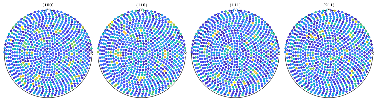
Plot estimated pole figures
plotPDF(rec,pf.h,'antipodal')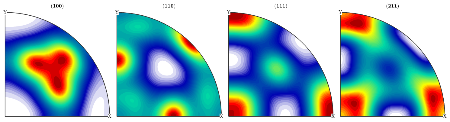
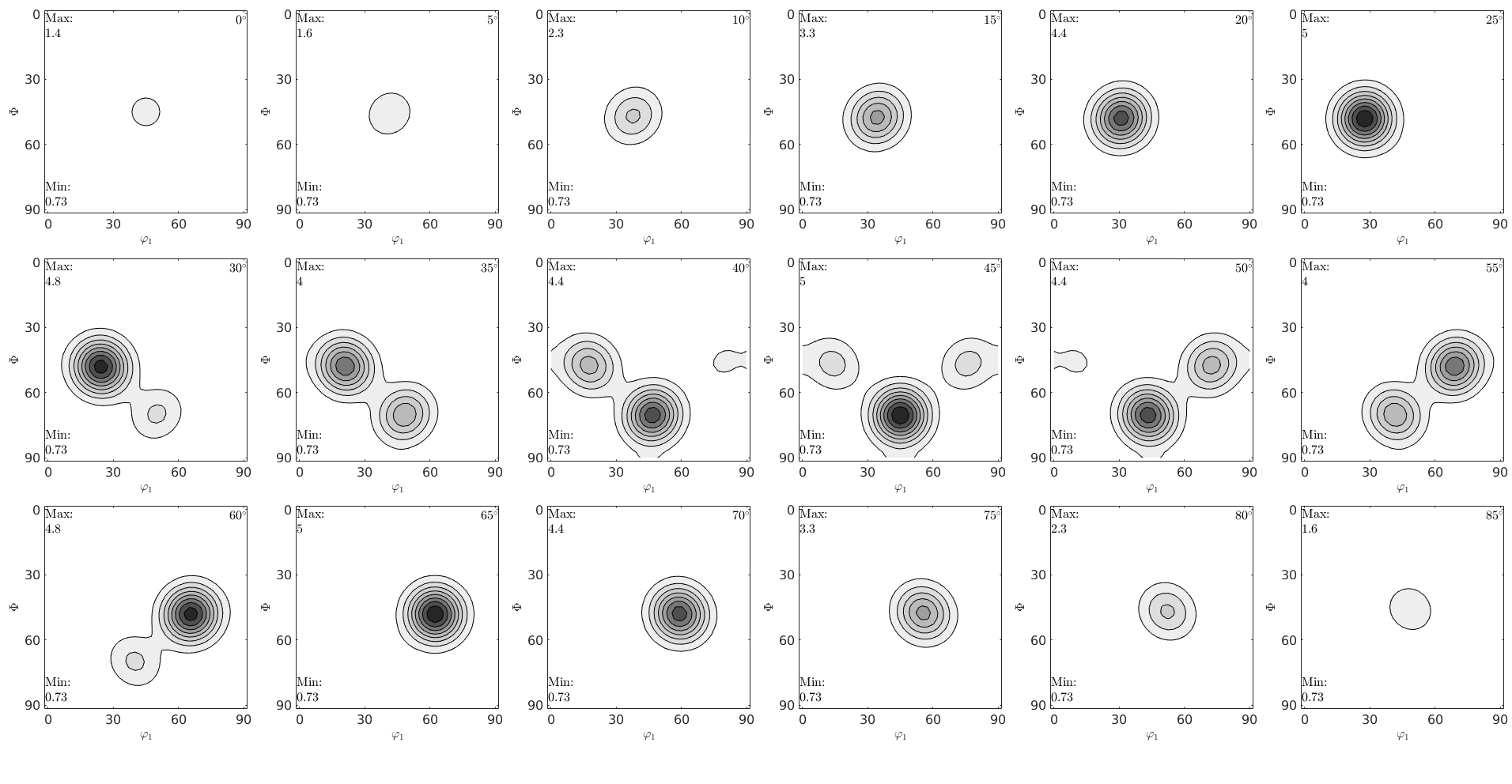
Plot estimated ODF (Ghost Corrected)
plot(rec,'sections',18,'resolution',5*degree,...
  'contourf','FontSize',10,'silent','figSize','large','minmax')
mtexColorMap white2black
progress: 100%
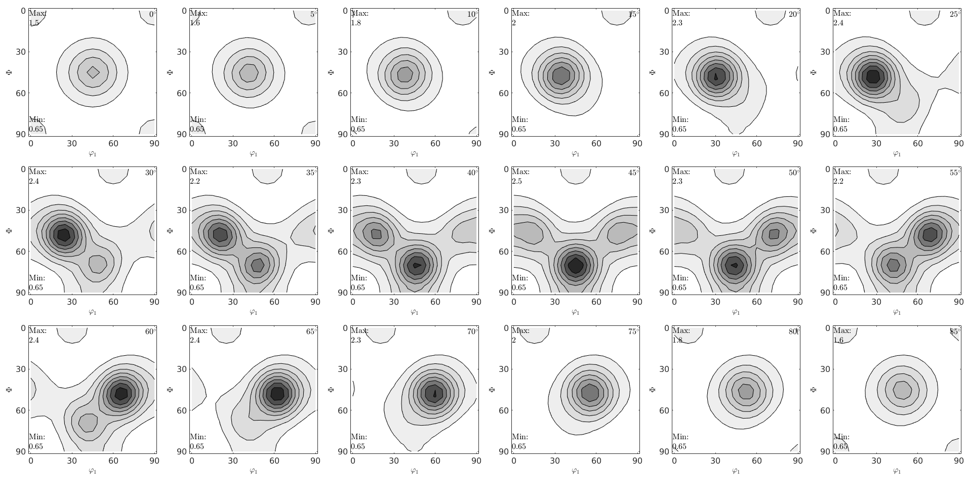
Plot odf
plot(SantaFe,'sections',18,'contourf','FontSize',10,'silent',...
  'figSize','large','minmax')
mtexColorMap white2black
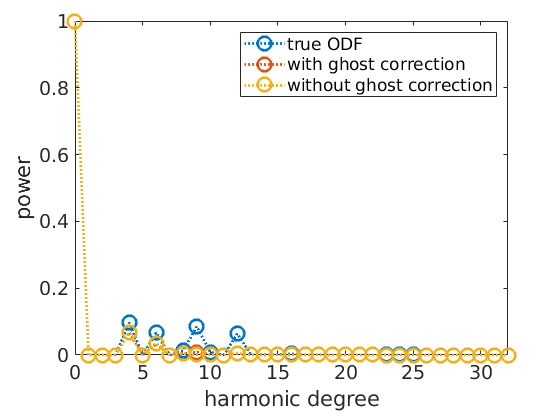
Plot Fourier Coefficients
close all;
% true ODF
plotFourier(SantaFe,'bandwidth',32,'linewidth',2)
% keep plot for adding the next plots
hold all

% With ghost correction:
plotFourier(rec,'bandwidth',32,'linewidth',2)

% Without ghost correction:
plotFourier(rec2,'bandwidth',32,'linewidth',2)

legend({'true ODF','with ghost correction','without ghost correction'})
% next plot command overwrites plot
hold off
| DocHelp 0.1 beta |