Plotting of Pole Figures
Describes various possibilities to visualize pole figure data.
| On this page ... |
| Import of Pole Figures |
| Visualize the Data |
| Contour Plots |
| Plotting Recalculated Pole Figures |
Import of Pole Figures
Let us start by loading some pole figures.
mtexdata ptxloading data ... saving data to /home/hielscher/mtex/master/data/ptx.mat
Visualize the Data
By default MTEX plots pole figures by drawing a circle at every measurement position of a pole figure and coloring it corresponding to the measured intensity.
plot(pf)
mtexColorbar
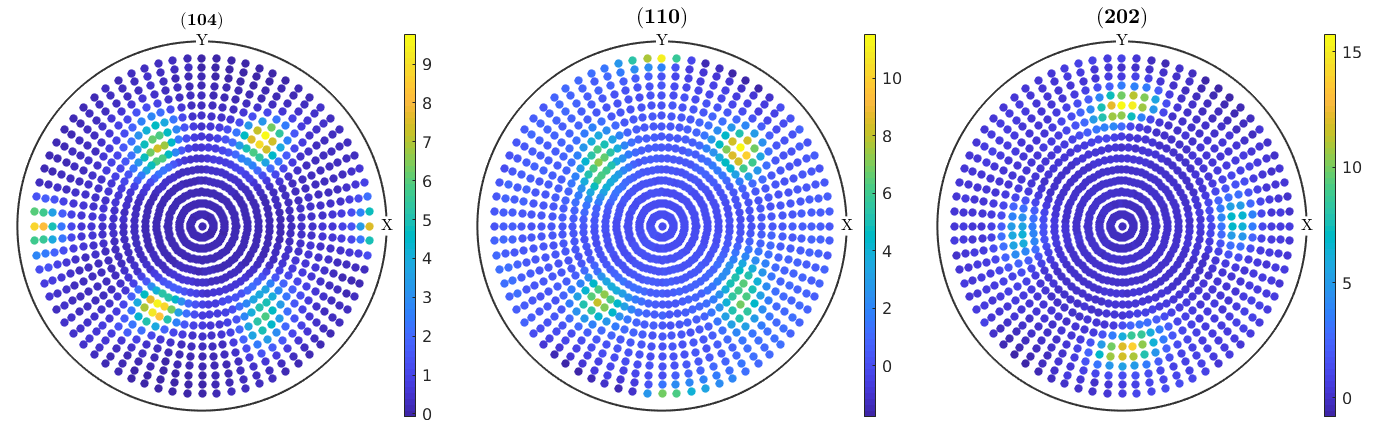
MTEX tries to guess the right size of the circle in order to produce a pleasing result. However, you can adjust this size using the option MarkerSize.
plot(pf,'MarkerSize',4)
mtexColorbar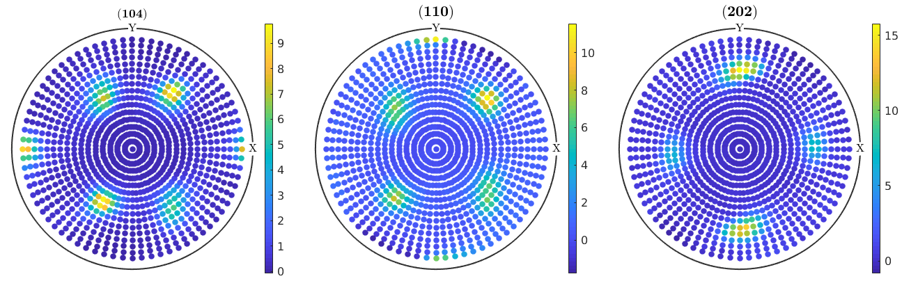
Contour Plots
Some people like to have their raw pole figures to be drawn as contour plots. This feature is not yet generally supported by MTEX. Note that measured pole figure may be given at a very irregular grid which would make it necessary to interpolate before drawing contours. In this case, however, it seems to be more reasonable to first compute an ODF and than to draw contour plots of the recalculated pole figures.
Nevertheless, MTEX offers basic contour plots in the case of regular measurement grids.
plot(pf,'contourf')
mtexColorbar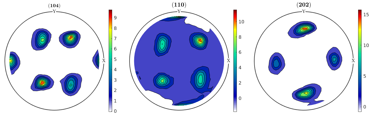
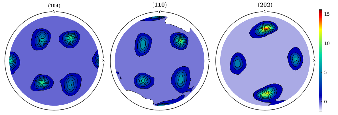
When drawing a colorbar next to the pole figure plots it is necessary to have the same color coding in all plots. This can be done as following
mtexColorbar % remove colorbars
CLim(gcm,'equal');
mtexColorbar % add a single colorbar
Plotting Recalculated Pole Figures
In order to draw recalculated one first needs to compute an ODF.
odf = calcODF(pf,'silent')
odf = ODF
  crystal symmetry : mmm
  specimen symmetry: -1

  Radially symmetric portion:
    kernel: de la Vallee Poussin, halfwidth 10°
    center: 29690 orientations, resolution: 5°
    weight: 1
Now smooth pole figures can be plotted for arbitrary crystallographic directions.
plotPDF(odf,pf.h,'antipodal')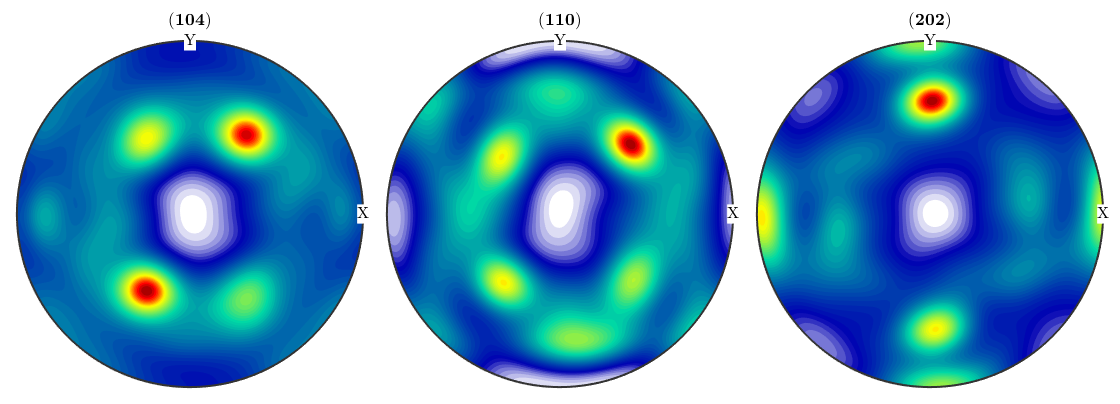
| DocHelp 0.1 beta |