The Piezoelectricity Tensor
how to work with piezoelectricity
This m-file mainly demonstrates how to illustrate the directional magnitude of a tensor with mtex
| On this page ... |
| Plotting the magnitude surface |
| Mean Tensor Calculation |
at first, let us import some piezoelectric contents for a quartz specimen.
CS = crystalSymmetry('32', [4.916 4.916 5.4054], 'X||a*', 'Z||c', 'mineral', 'Quartz');

fname = fullfile(mtexDataPath,'tensor', 'Single_RH_quartz_poly.P');

P = tensor.load(fname,CS,'propertyname','piecoelectricity','unit','C/N','DoubleConvention')
P = tensor
  propertyname    : piecoelectricity
  unit            : C/N
  rank            : 3 (3 x 3 x 3)
  doubleConvention: true
  mineral         : Quartz (321, X||a*, Y||b, Z||c*)

  tensor in compact matrix form:
     0     0     0 -0.67     0   4.6
   2.3  -2.3     0     0  0.67     0
     0     0     0     0     0     0
Plotting the magnitude surface
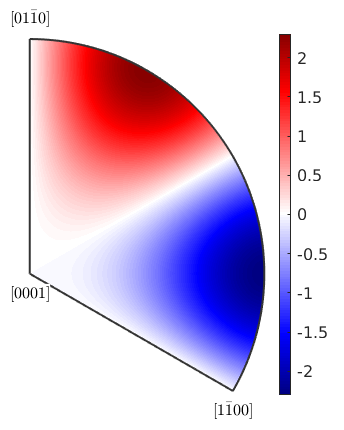
The default plot of the magnitude, which indicates, in which direction we have the most polarization. By default, we restrict ourselves to the unique region implied by crystal symmetry
% set some colormap well suited for tensor visualisation
setMTEXpref('defaultColorMap',blue2redColorMap);

plot(P)
mtexColorbar
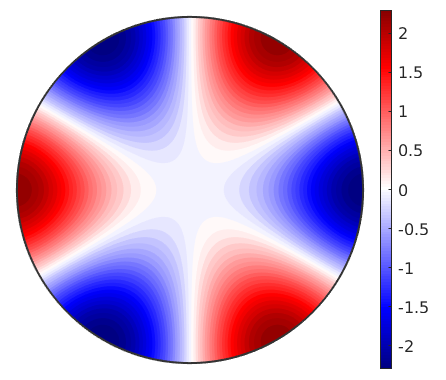
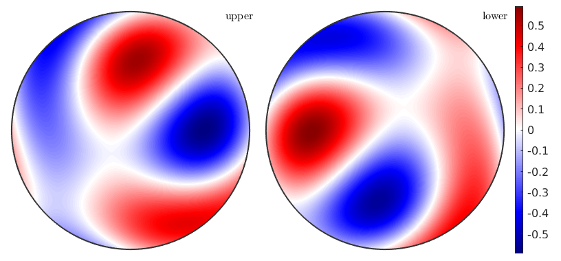
but also, we can plot the whole crystal behavior
close all
plot(P,'complete','smooth','upper')
mtexColorbar
Most often, the polarization is illustrated as surface magnitude
close all
surf(P.directionalMagnitude)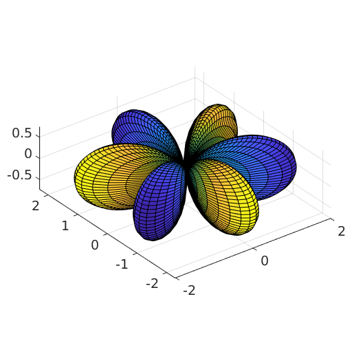
Note, that for directions of negative polarization the surface is mapped onto the axis of positive, which then let the surface appear as a double coverage
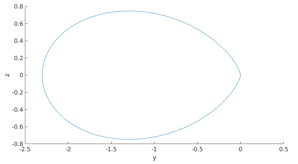
Quite a famous example in various standard literature is a section through the surface because it can easily be described as an analytical solution. We just specify the plane normal vector
plotSection(P.directionalMagnitude,vector3d.Z)
xlabel('x')
ylabel('y')
drawNow(gcm)
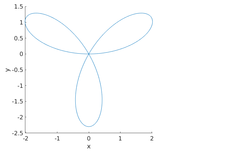
so we are plotting the polarization in the xy-plane, or the yz-plane with
plotSection(P.directionalMagnitude,vector3d.X)
ylabel('y')
zlabel('z')
drawNow(gcm)
Mean Tensor Calculation
Let us import some data, which was originally published by Mainprice, D., Lloyd, G.E. and Casey , M. (1993) Individual orientation measurements in quartz polycrystals: advantages and limitations for texture and petrophysical property determinations. J. of Structural Geology, 15, pp.1169-1187
fname = fullfile(mtexDataPath,'orientation', 'Tongue_Quartzite_Bunge_Euler');

ori = loadOrientation(fname,CS,'interface','generic' ...
  , 'ColumnNames', { 'Euler 1' 'Euler 2' 'Euler 3'}, 'Bunge', 'active rotation')
ori = orientation
  size: 382 x 1
  crystal symmetry : Quartz (321, X||a*, Y||b, Z||c*)
  specimen symmetry: 1
The figure on p.1184 of the publication
Pm = ori.calcTensor(P)

plot(Pm)
mtexColorbar
Pm = tensor
  propertyname    : piecoelectricity
  unit            : C/N
  rank            : 3 (3 x 3 x 3)
  doubleConvention: true

  tensor in compact matrix form: *10^-2
 -10.48   34.2 -23.72 -32.75 -64.24 -26.18
 -18.02  -3.15  21.17  62.42  29.67  44.39
 -41.35  40.44   0.91  32.48 -23.42   6.47

close all
plot(Pm)
mtexColorbar

setMTEXpref('defaultColorMap',WhiteJetColorMap)
| DocHelp 0.1 beta |