Orientation Density Functions
This example demonstrates the most important MTEX tools for analysing ODFs.
All described commands can be applied to model ODFs constructed via uniformODF, unimodalODF, or fibreODF and to all estimated ODF calculated from pole figures or EBSD data.
Defining Model ODFs
Unimodal ODFs
SS  = specimenSymmetry('orthorhombic');
CS  = crystalSymmetry('cubic');
o   = orientation.brass(CS,SS);
psi = vonMisesFisherKernel('halfwidth',20*degree);

odf1 = unimodalODF(o,CS,SS,psi)
odf1 = ODF
  crystal symmetry : m-3m
  specimen symmetry: mmm

  Radially symmetric portion:
    kernel: van Mises Fisher, halfwidth 20°
    center: (35°,45°,0°)
    weight: 1
Fibre ODFs
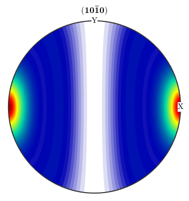
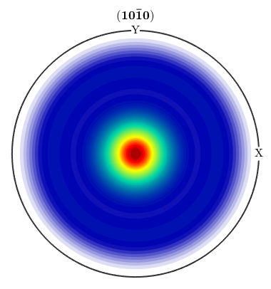
CS = crystalSymmetry('hexagonal');
h = Miller(1,0,0,CS);
r = xvector;
psi = AbelPoissonKernel('halfwidth',18*degree);

odf2 = fibreODF(h,r,psi)
odf2 = ODF
  crystal symmetry : 6/mmm, X||a*, Y||b, Z||c*
  specimen symmetry: 1

  Fibre symmetric portion:
    kernel: Abel Poisson, halfwidth 18°
    fibre: (10-10) - 1,0,0
    weight: 1
uniform ODFs
odf3 = uniformODF(CS)
odf3 = ODF
  crystal symmetry : 6/mmm, X||a*, Y||b, Z||c*
  specimen symmetry: 1

  Uniform portion:
    weight: 1
FourierODF
Bingham ODFs
Lambda = [-10,-10,10,10]
A = quaternion(eye(4))
odf = BinghamODF(Lambda,A,CS)

plotIPDF(odf,xvector)
plotPDF(odf,Miller(1,0,0,CS))
Lambda =
   -10   -10    10    10

A = Quaternion
  size: 1 x 4
  a b c d
  1 0 0 0
  0 1 0 0
  0 0 1 0
  0 0 0 1

odf = ODF
  crystal symmetry : 6/mmm, X||a*, Y||b, Z||c*
  specimen symmetry: 1

  Bingham portion:
     kappa: -10 -10 10 10
    weight: 1
ODF Arithmetics
0.3*odf2 + 0.7*odf3

rot = rotation.byAxisAngle(yvector,90*degree);
odf = rotate(odf,rot)
plotPDF(odf,Miller(1,0,0,CS))
ans = ODF
  crystal symmetry : 6/mmm, X||a*, Y||b, Z||c*
  specimen symmetry: 1

  Fibre symmetric portion:
    kernel: Abel Poisson, halfwidth 18°
    fibre: (10-10) - 1,0,0
    weight: 0.3

  Uniform portion:
    weight: 0.7


odf = ODF
  crystal symmetry : 6/mmm, X||a*, Y||b, Z||c*
  specimen symmetry: 1

  Bingham portion:
     kappa: -10 -10 10 10
    weight: 1
Working with ODFs
% *Texture Characteristics+

calcError(odf2,odf3,'L1')      % difference between ODFs

[maxODF,centerODF] = max(odf)  % the modal orientation
mean(odf)                      % the mean orientation
max(odf)

volume(odf,centerODF,5*degree) % the volume of a ball
fibreVolume(odf2,h,r,5*degree) % the volume of a fibre

textureindex(odf)              % the texture index
entropy(odf)                   % the entropy
f_hat = calcFourier(odf2,16);  % the C-coefficients up to order 16
ans =
    0.2030
maxODF =
    3.3783

centerODF = orientation
  size: 1 x 1
  crystal symmetry : 6/mmm, X||a*, Y||b, Z||c*
  specimen symmetry: 1

  Bunge Euler angles in degree
  phi1  Phi phi2 Inv.
    90   90  270    0


ans = orientation
  size: 1 x 1
  crystal symmetry : 6/mmm, X||a*, Y||b, Z||c*
  specimen symmetry: 1

  Bunge Euler angles in degree
     phi1         Phi        phi2        Inv.
  106.893 0.000738512     251.926           0

ans =
    3.3783
ans =
    0.0028
ans =
    0.0253
ans =
    1.9251
ans =
   -0.5028
Plotting ODFs
Plotting (Inverse) Pole Figures
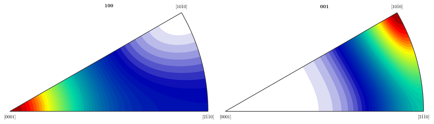
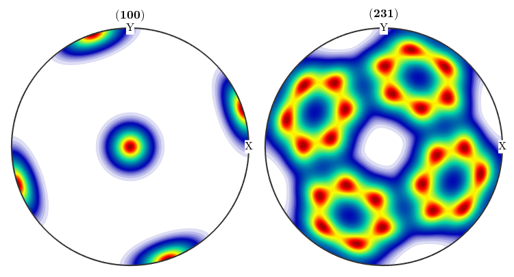
close all
plotPDF(odf,Miller(0,1,0,CS),'antipodal')
plotIPDF(odf,[xvector,zvector])
Plotting an ODF
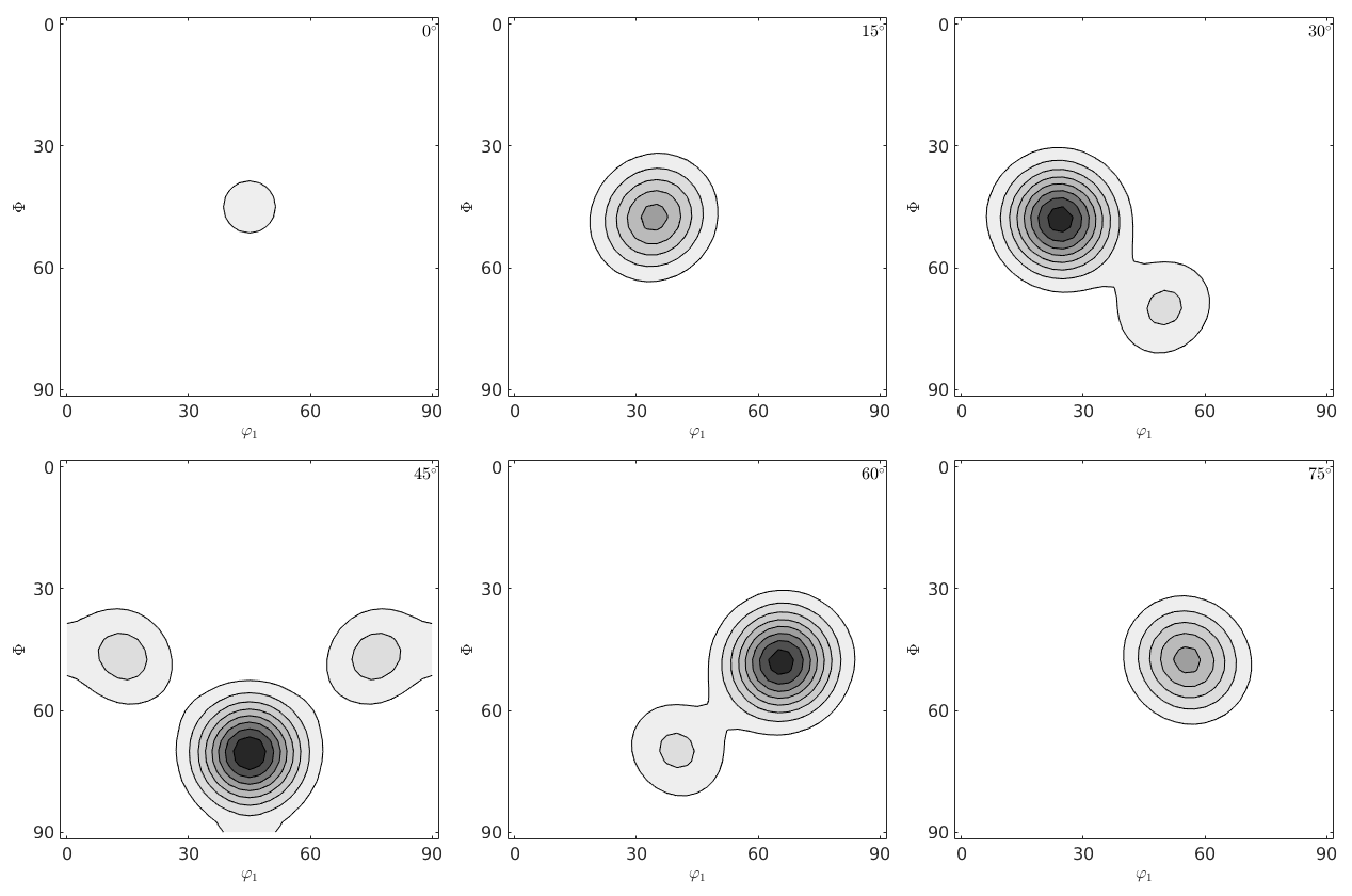
close all
plot(SantaFe,'alpha','sections',6,'projection','plain','contourf')
mtexColorMap white2black
Exercises
2)
a) Construct a cubic unimodal ODF with mod at [0 0 1](3 1 0). (Miller indice). What is its modal orientation in Euler angles?
CS = crystalSymmetry('cubic');
ori = orientation.byMiller([0 0 1],[3 1 0],CS);
odf = unimodalODF(ori);
b) Plot some pole figures. Are there pole figures with and without antipodal symmetry? What about the inverse pole figures?
plotPDF(odf,[Miller(1,0,0,CS),Miller(2,3,1,CS)])
close all;plotPDF(odf,[Miller(1,0,0,CS),Miller(2,3,1,CS)],'antipodal')
close all;plotIPDF(odf,vector3d(1,1,3))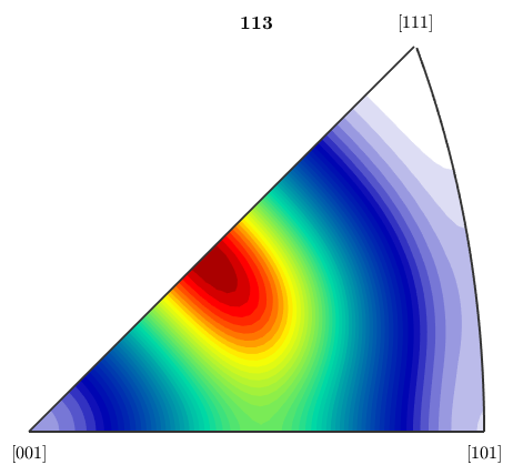
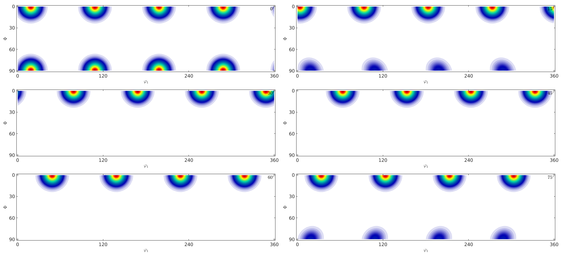
c) Plot the ODF in sigma and phi2 - sections. How many mods do you observe?
close all; plot(odf,'sections',6)
d) Compute the volume of the ODF that is within a distance of 10 degree of the mod. Compare to an the uniform ODF.
volume(odf,ori,10*degree)
volume(uniformODF(CS,SS),ori,10*degree)
ans =
    0.2939
ans =
    0.0269
e) Construct a trigonal ODF that consists of two fibres at h1 = (0,0,0,1), r1 = (0,1,0), h2 = (1,0,-1,0), r2 = (1,0,0). Do the two fibres intersect?
cs = crystalSymmetry('trigonal');
odf = 0.5 * fibreODF(Miller(0,0,0,1,cs),yvector) + ...
      0.5 * fibreODF(Miller(1,0,-1,0,cs),xvector)
odf = ODF
  crystal symmetry : -31m, X||a*, Y||b, Z||c*
  specimen symmetry: 1

  Fibre symmetric portion:
    kernel: de la Vallee Poussin, halfwidth 10°
    fibre: (0001) - 0,1,0
    weight: 0.5

  Fibre symmetric portion:
    kernel: de la Vallee Poussin, halfwidth 10°
    fibre: (10-10) - 1,0,0
    weight: 0.5
f) What is the modal orientation of the ODF?
mod = calcModes(odf)
mod = orientation
  size: 1 x 1
  crystal symmetry : -31m, X||a*, Y||b, Z||c*
  specimen symmetry: 1

  Bunge Euler angles in degree
  phi1  Phi phi2 Inv.
   180   90  180    0
g) Plot the ODF in sigma and phi2 - sections. How many fibre do you observe?
close all;plot(odf,'sections',6)
mtexColorMap white2black
annotate(mod,'MarkerColor','r','Marker','s')
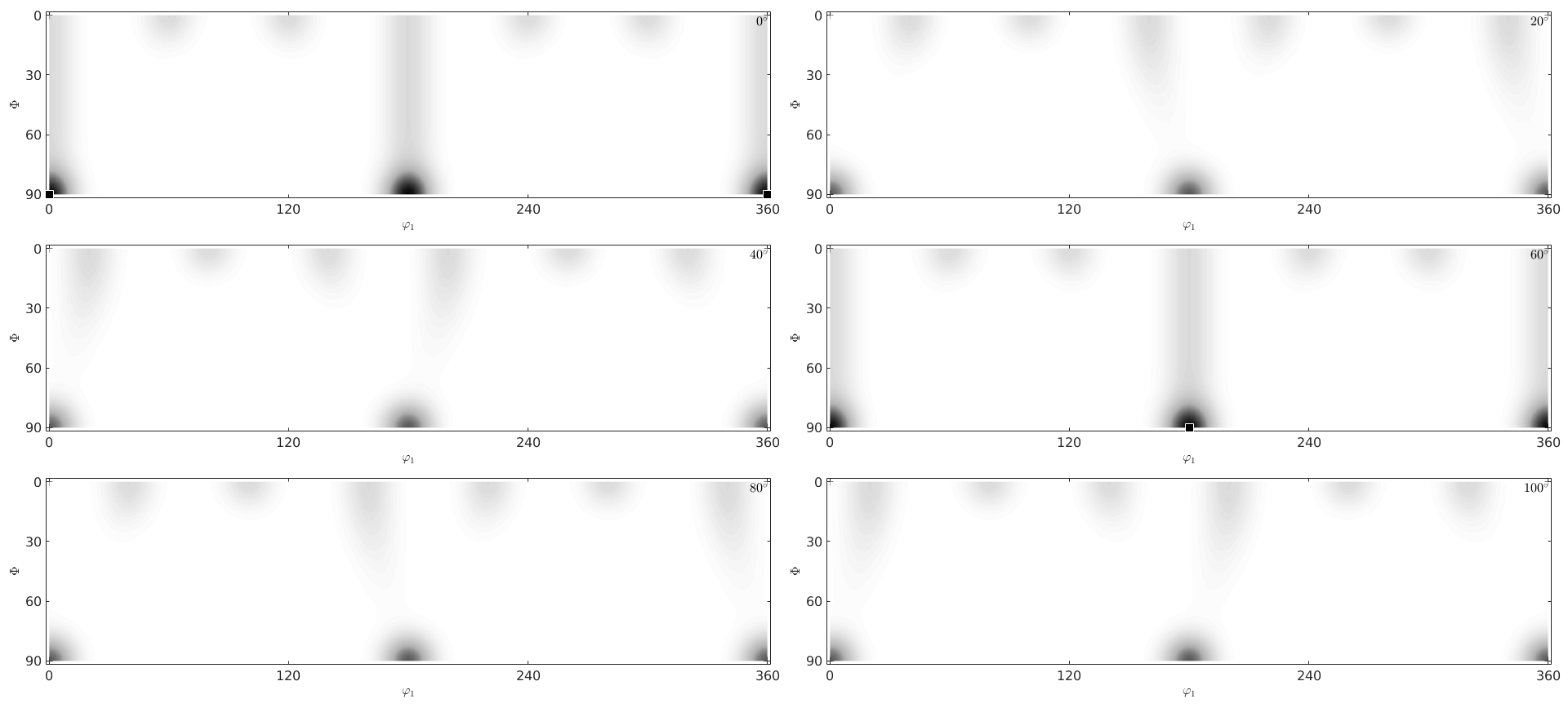
plot(odf,'phi2','sections',6)

h) Compute the texture index of the ODF.
textureindex(odf)
ans =
    9.6324
| DocHelp 0.1 beta |