Misorientations
Misorientation describes the relative orientation of two grains with respect to each other. Important concepts are twinnings and CSL (coincidence site lattice),
| On this page ... |
| The misorientation angle |
| Misorientations |
| Coincident lattice planes |
| Twinning misorientations |
| Highlight twinning boundaries |
| Phase transitions |
The misorientation angle
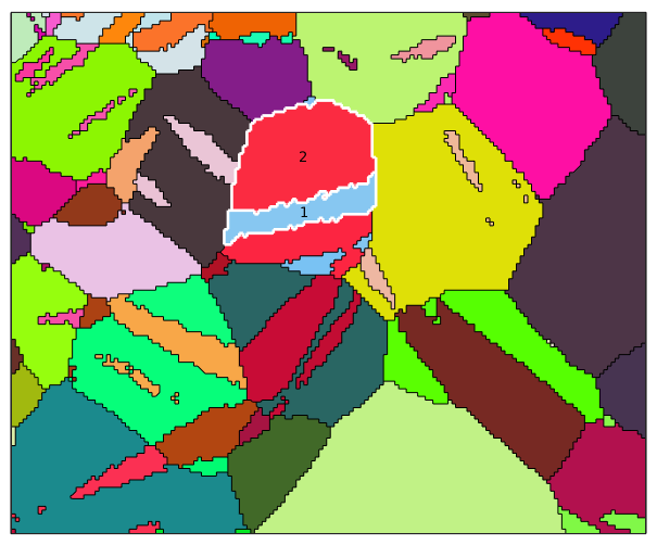
First we import some EBSD data set, compute grains and plot them according to their mean orientation. Next we highlight grain 70 and grain 80
mtexdata twins
% use only proper symmetry operations
ebsd('M').CS = ebsd('M').CS.properGroup;
grains = calcGrains(ebsd('indexed'),'threshold',5*degree)
CS = grains.CS; % extract crystal symmetry

plot(grains,grains.meanOrientation,'micronbar','off')
hold on
plot(grains([74,85]).boundary,'edgecolor','w','linewidth',2)

text(grains([74,85]),{'1','2'})
grains = grain2d

 Phase  Grains  Pixels    Mineral  Symmetry  Crystal reference frame
     1     126   22833  Magnesium       622       X||a*, Y||b, Z||c*

 boundary segments: 3892
 triple points: 122

 Properties: GOS, meanRotation

  I'm going to colorize the orientation data with the
  standard MTEX colorkey. To view the colorkey do:

  colorKey = ipfColorKey(ori_variable_name)
  plot(colorKey)
After extracting the mean orientation of grain 70 and 80
ori1 = grains(74).meanOrientation
ori2 = grains(85).meanOrientation
ori1 = orientation
  size: 1 x 1
  crystal symmetry : Magnesium (622, X||a*, Y||b, Z||c*)
  specimen symmetry: 1

  Bunge Euler angles in degree
     phi1     Phi    phi2    Inv.
  19.4774 78.0484 220.043       0


ori2 = orientation
  size: 1 x 1
  crystal symmetry : Magnesium (622, X||a*, Y||b, Z||c*)
  specimen symmetry: 1

  Bunge Euler angles in degree
     phi1     Phi    phi2    Inv.
  71.4509 167.781 200.741       0
we may compute the misorientation angle between both orientations by
angle(ori1, ori2) ./ degree
ans =
   85.7093
Note that the misorientation angle is computed by default modulo crystal symmetry, i.e., the angle is always the smallest angles between all possible pairs of symmetrically equivalent orientations. In our example this means that symmetrisation of one orientation has no impact on the angle
angle(ori1, ori2.symmetrise) ./ degree
ans =
   85.7093
   85.7093
   85.7093
   85.7093
   85.7093
   85.7093
   85.7093
   85.7093
   85.7093
   85.7093
   85.7093
   85.7093
The misorientation angle neglecting crystal symmetry can be computed by
angle(ori1, ori2.symmetrise,'noSymmetry')./ degreeans = 107.9464 100.9175 94.2925 136.6180 107.7066 179.5952 140.0598 137.3717 179.8061 101.4414 140.4168 85.7093
We see that the smallest angle indeed coincides with the angle computed before.
Misorientations
Remember that both orientations ori1 and ori2 map crystal coordinates onto specimen coordinates. Hence, the product of an inverse orientation with another orientation transfers crystal coordinates from one crystal reference frame into crystal coordinates with respect to another crystal reference frame. This transformation is called misorientation
mori = inv(ori1) * ori2
mori = misorientation
  size: 1 x 1
  crystal symmetry : Magnesium (622, X||a*, Y||b, Z||c*)
  crystal symmetry : Magnesium (622, X||a*, Y||b, Z||c*)

  Bunge Euler angles in degree
     phi1     Phi    phi2    Inv.
  149.581 94.2922 150.134       0
In the present case the misorientation describes the coordinate transform from the reference frame of grain 80 into the reference frame of crystal 70. Take as an example the plane {11-20} with respect to the grain 80. Then the plane in grain 70 which alignes parallel to this plane can be computed by
round(mori * Miller(1,1,-2,0,CS))
ans = Miller
 size: 1 x 1
 mineral: Magnesium (622, X||a*, Y||b, Z||c*)
  h  2
  k -1
  i -1
  l  0
Conversely, the inverse of mori is the coordinate transform from crystal 70 to grain 80.
round(inv(mori) * Miller(2,-1,-1,0,CS))
ans = Miller
 size: 1 x 1
 mineral: Magnesium (622, X||a*, Y||b, Z||c*)
  h  1
  k  1
  i -2
  l  0
Coincident lattice planes
The coincidence between major lattice planes may suggest that the misorientation is a twinning misorientation. Lets analyse whether there are some more alignments between major lattice planes.
%m = Miller({1,-1,0,0},{1,1,-2,0},{1,-1,0,1},{0,0,0,1},CS);
m = Miller({1,-1,0,0},{1,1,-2,0},{-1,0,1,1},{0,0,0,1},CS);

% cycle through all major lattice planes
close all
for im = 1:length(m)
  % plot the lattice planes of grains 80 with respect to the
  % reference frame of grain 70
  plot(mori * m(im).symmetrise,'MarkerSize',10,...
    'DisplayName',char(m(im)),'figSize','large','noLabel','upper')
  hold all
end
hold off

% mark the corresponding lattice planes in the twin
mm = round(unique(mori*m.symmetrise,'noSymmetry'),'maxHKL',6);
annotate(mm,'labeled','MarkerSize',5,'figSize','large','textAboveMarker')

% show legend
legend({},'location','SouthEast','FontSize',13);
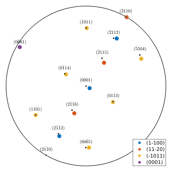
we observe an almost perfect match for the lattice planes {11-20} to {-2110} and {1-101} to {-1101} and good coincidences for the lattice plane {1-100} to {0001} and {0001} to {0-661}. Lets compute the angles explicitly
angle(mori * Miller(1,1,-2,0,CS),Miller(2,-1,-1,0,CS)) / degree
angle(mori * Miller(1,0,-1,-1,CS),Miller(1,-1,0,1,CS)) / degree
angle(mori * Miller(0,0,0,1,CS) ,Miller(1,0,-1,0,CS),'noSymmetry') / degree
angle(mori * Miller(1,1,-2,2,CS),Miller(1,0,-1,0,CS)) / degree
angle(mori * Miller(1,0,-1,0,CS),Miller(1,1,-2,2,CS)) / degree
ans =
0.4489
ans =
0.2193
ans =
59.6757
ans =
2.6092
ans =
2.5387
Twinning misorientations
Lets define a misorientation that makes a perfect fit between the {11-20} lattice planes and between the {10-11} lattice planes
mori = orientation.map(Miller(1,1,-2,0,CS),Miller(2,-1,-1,0,CS),...
  Miller(-1,0,1,1,CS),Miller(-1,1,0,1,CS))


% the rotational axis
round(mori.axis)

% the rotational angle
mori.angle / degree
mori = misorientation
  size: 1 x 1
  crystal symmetry : Magnesium (622, X||a*, Y||b, Z||c*)
  crystal symmetry : Magnesium (622, X||a*, Y||b, Z||c*)

  Bunge Euler angles in degree
  phi1  Phi phi2 Inv.
   300    0    0    0


ans = Miller
 size: 1 x 1
 mineral: Magnesium (622, X||a*, Y||b, Z||c*)
  h  1
  k  0
  i -1
  l  0
ans =
     0
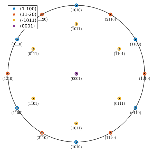
and plot the same figure as before with the exact twinning misorientation.
% cycle through all major lattice planes
close all
for im = 1:length(m)
  % plot the lattice planes of grains 80 with respect to the
  % reference frame of grain 70
  plot(mori * m(im).symmetrise,'MarkerSize',10,...
    'DisplayName',char(m(im)),'figSize','large','noLabel','upper')
  hold all
end
hold off

% mark the corresponding lattice planes in the twin
mm = round(unique(mori*m.symmetrise,'noSymmetry'),'maxHKL',6);
annotate(mm,'labeled','MarkerSize',5,'figSize','large')

% show legend
legend({},'location','NorthWest','FontSize',13);
Highlight twinning boundaries
It turns out that in the previous EBSD map many grain boundaries have a misorientation close to the twinning misorientation we just defined. Lets Lets highlight those twinning boundaries
% consider only Magnesium to Magnesium grain boundaries
gB = grains.boundary('Mag','Mag');

% check for small deviation from the twinning misorientation
isTwinning = angle(gB.misorientation,mori) < 5*degree;

% plot the grains and highlight the twinning boundaries
plot(grains,grains.meanOrientation,'micronbar','off')
hold on
plot(gB(isTwinning),'edgecolor','w','linewidth',2)
hold off
  I'm going to colorize the orientation data with the
  standard MTEX colorkey. To view the colorkey do:

  colorKey = ipfColorKey(ori_variable_name)
  plot(colorKey)
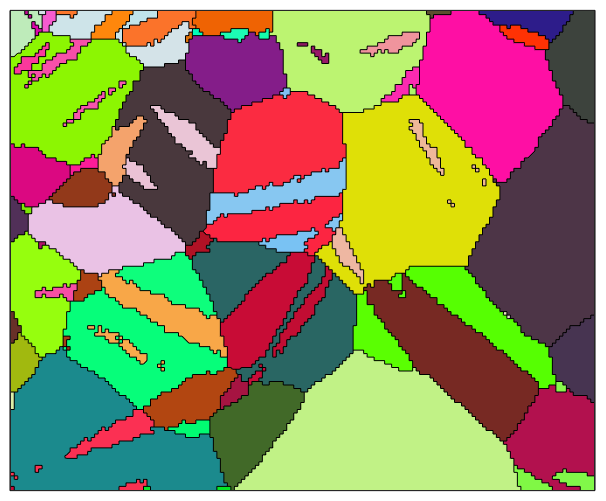
From this picture we see that large fraction of grain boudaries are twinning boundaries. To make this observation more evident we may plot the boundary misorientation angle distribution function. This is simply the angle distribution of all boundary misorientations and can be displayed with
close all
plotAngleDistribution(gB.misorientation)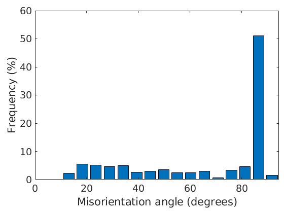
From this we observe that we have about 50 percent twinning boundaries. Analogously we may also plot the axis distribution
plotAxisDistribution(gB.misorientation,'contour')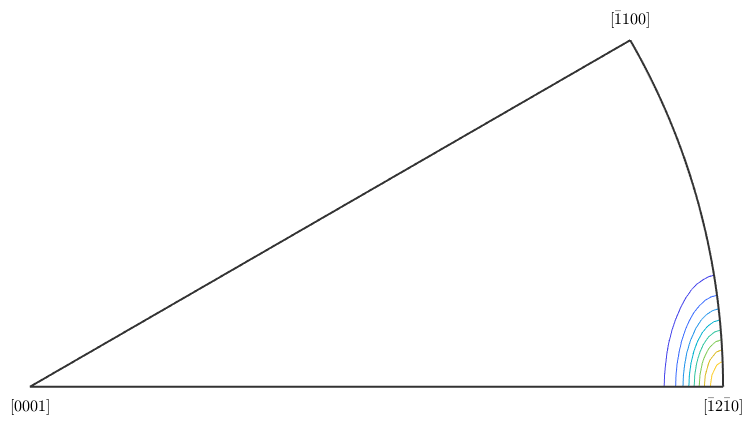
which emphasises a strong portion of rotations about the (-12-10) axis.
Phase transitions
Misorientations may not only be defined between crystal frames of the same phase. Lets consider the phases Magnetite and Hematite.
CS_Mag = loadCIF('Magnetite')
CS_Hem = loadCIF('Hematite')
CS_Mag = crystalSymmetry

  mineral : Magnetite
  symmetry: m-3m
  a, b, c : 8.4, 8.4, 8.4


CS_Hem = crystalSymmetry

  mineral        : Hematite
  symmetry       : -3m1
  a, b, c        : 5, 5, 14
  reference frame: X||a*, Y||b, Z||c*
The phase transition from Magnetite to Hematite is described in literature by {111}_m parallel {0001}_h and {-101}_m parallel {10-10}_h The corresponding misorientation is defined in MTEX by
Mag2Hem = orientation.map(...
  Miller(1,1,1,CS_Mag),Miller(0,0,0,1,CS_Hem),...
  Miller(-1,0,1,CS_Mag),Miller(1,0,-1,0,CS_Hem))
Mag2Hem = misorientation
  size: 1 x 1
  crystal symmetry : Magnetite (m-3m)
  crystal symmetry : Hematite (-3m1, X||a*, Y||b, Z||c*)

  Bunge Euler angles in degree
  phi1     Phi    phi2    Inv.
   120 54.7356      45       0
Assume a Magnetite grain with orientation
ori_Mag = orientation.byEuler(0,0,0,CS_Mag)
ori_Mag = orientation
  size: 1 x 1
  crystal symmetry : Magnetite (m-3m)
  specimen symmetry: 1

  Bunge Euler angles in degree
  phi1  Phi phi2 Inv.
     0    0    0    0
Then we can compute all variants of the phase transition by
symmetrise(ori_Mag) * inv(Mag2Hem)
ans = orientation
  size: 48 x 1
  crystal symmetry : Hematite (-3m1, X||a*, Y||b, Z||c*)
  specimen symmetry: 1
and the corresponding pole figures by
plotPDF(symmetrise(ori_Mag) * inv(Mag2Hem),...
  Miller({1,0,-1,0},{1,1,-2,0},{0,0,0,1},CS_Hem))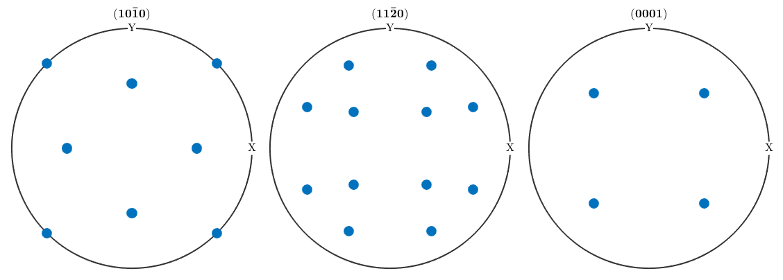
| DocHelp 0.1 beta |