Misorientation Distribution Function

Computing a misorientation distribution function from EBSD data

Lets import some EBSD data and reconstruct the grains.

mtexdata forsterite
grains = calcGrains(ebsd)

 
grains = grain2d  
 
 Phase  Grains  Pixels     Mineral  Symmetry  Crystal reference frame
     0   16334   58485  notIndexed                                   
     1    4092  152345  Forsterite       mmm                         
     2    1864   26058   Enstatite       mmm                         
     3    1991    9064    Diopside     12/m1       X||a*, Y||b*, Z||c
 
 boundary segments: 147957
 triple points: 11456
 
 Properties: GOS, meanRotation
 

Back to Top

The boundary misorientation distribution function

The boundary misorientation distribution function for the phase transition from Forsterite to Enstatite can be computed by

mdf_boundary = calcODF(grains.boundary('Fo','En').misorientation,'halfwidth',10*degree)

 
mdf_boundary = MDF  
  crystal symmetry : Forsterite (mmm)
  crystal symmetry : Enstatite (mmm)
 
  Harmonic portion:
    degree: 25
    weight: 1
 

The misorientation distribution function can be processed as any other ODF. E.g. we can compute the prefered misorientation via

[v,mori] = max(mdf_boundary)

v =
   38.8766
 
mori = misorientation  
  size: 1 x 1
  crystal symmetry : Forsterite (mmm)
  crystal symmetry : Enstatite (mmm)
 
  Bunge Euler angles in degree
     phi1     Phi    phi2    Inv.
  82.4065 1.06577 187.671       0
 

or plot the pole figure corresponding to the crystal axis (1,0,0)

plotPDF(mdf_boundary,Miller(1,0,0,ebsd('Fo').CS))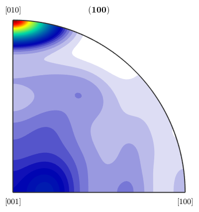

Back to Top

The uncorrelated misorientation distribution function

Alternatively the uncorrelated misorientation distribution function can be computed by providing the option uncorrelated

mori = calcMisorientation(ebsd('En'),ebsd('Fo'))
mdf_uncor = calcODF(mori)

 
mori = misorientation  
  size: 98541 x 1
  crystal symmetry : Forsterite (mmm)
  crystal symmetry : Enstatite (mmm)
 
 
mdf_uncor = MDF  
  crystal symmetry : Forsterite (mmm)
  crystal symmetry : Enstatite (mmm)
 
  Harmonic portion:
    degree: 25
    weight: 1
 

Obviously it is different from the boundary misorientation distribution function.

plotPDF(mdf_uncor,Miller(1,0,0,ebsd('Fo').CS))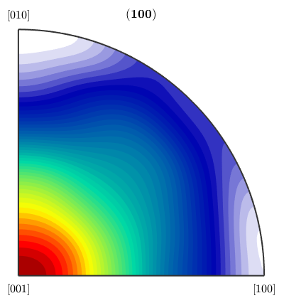

Back to Top

Computing the uncorrelated misorientation function from two ODFs

Let given two odfs

odf_fo = calcODF(ebsd('fo').orientations,'halfwidth',10*degree)
odf_en = calcODF(ebsd('en').orientations,'halfwidth',10*degree)

 
odf_fo = ODF  
  crystal symmetry : Forsterite (mmm)
  specimen symmetry: 1
 
  Harmonic portion:
    degree: 25
    weight: 1
 
 
odf_en = ODF  
  crystal symmetry : Enstatite (mmm)
  specimen symmetry: 1
 
  Harmonic portion:
    degree: 25
    weight: 1
 

Then the uncorrelated misorientation function between these two ODFs can be computed by

mdf = calcMDF(odf_en,odf_fo)

 
mdf = MDF  
  crystal symmetry : Forsterite (mmm)
  crystal symmetry : Enstatite (mmm)
 
  Harmonic portion:
    degree: 19
    weight: 1
 

This misorientation distribution function should be similar to the uncorrelated misorientation function computed directly from the ebsd data

plotPDF(mdf,Miller(1,0,0,ebsd('Fo').CS))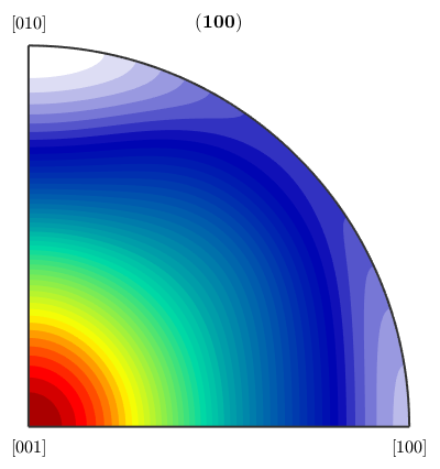

Back to Top

Analyzing misorientation functions

Back to Top

Angle distribution

Let us first compare the actual angle distribution of the boundary misorientations with the theoretical angle distribution of the uncorrelated MDF.

close all
plotAngleDistribution(grains.boundary('fo','en').misorientation)

hold on

plotAngleDistribution(mdf)

hold off

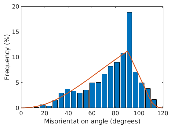
For computing the exact values see the commands calcAngleDistribution(mdf) and calcAngleDistribution(grains).

Back to Top

Axis distribution

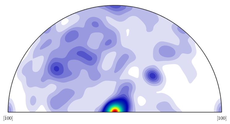
The same we can do with the axis distribution. First the actual angle distribution of the boundary misorientations

plotAxisDistribution(grains.boundary('fo','en').misorientation,'smooth')

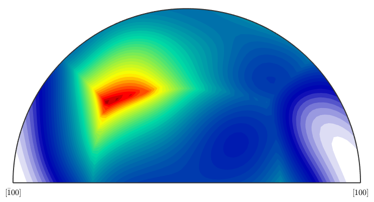
Now the theoretical axis distribution of the uncorrelated MDF.

plotAxisDistribution(mdf)

For computing the exact values see the commands calcAxisDistribution(mdf) and calcAxisDistribution(grains).

Back to Top

DocHelp 0.1 beta