Working with Grains
How to index grains and access shape properties.
| On this page ... |
| Accessing individual grains |
| Indexing by a Condition |
| Indexing by orientation or position |
| Grain-size Analysis |
| Spatial Dependencies |
Grains have several intrinsic properties, which can be used for statistical, shape as well as for spatial analysis
Let us first import some EBSD data and reconstruct grains
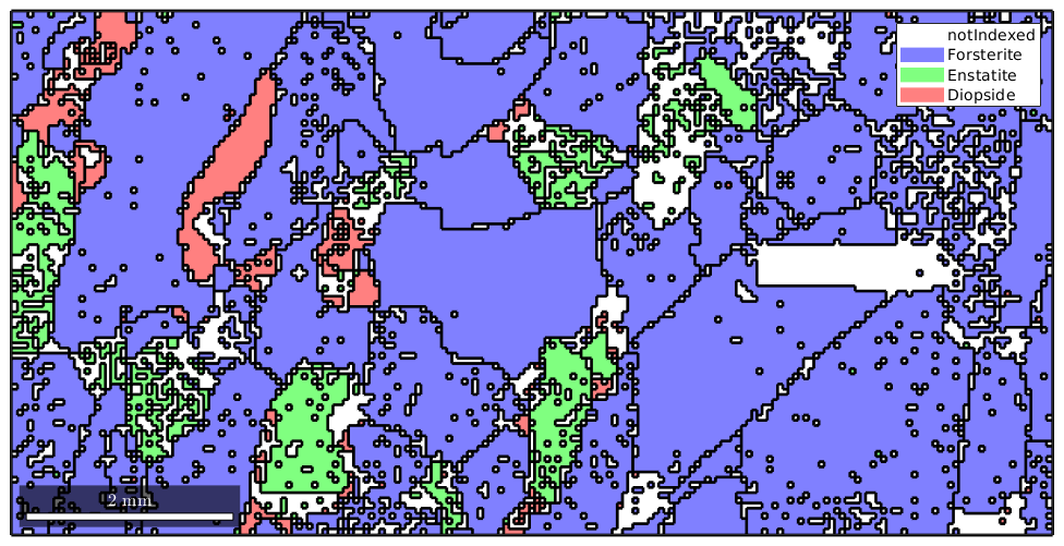
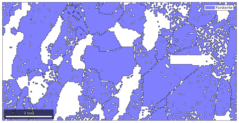
plotx2east
mtexdata forsterite
ebsd = ebsd(inpolygon(ebsd,[5 2 10 5]*10^3));
grains = calcGrains(ebsd)

plot(ebsd)
hold on
plot(grains.boundary,'linewidth',2)
hold off
grains = grain2d

 Phase  Grains  Pixels     Mineral  Symmetry  Crystal reference frame
     0    1139    4052  notIndexed
     1     242   14093  Forsterite       mmm
     2     177    1397   Enstatite       mmm
     3     104     759    Diopside     12/m1       X||a*, Y||b*, Z||c

 boundary segments: 10420
 triple points: 903

 Properties: GOS, meanRotation
Accessing individual grains
The variable grains is essentially a large vector of grains. Thus when applying a function like area to this variable we obtain a vector of the same lenght with numbers representing the area of each grain
grain_area = grains.area;
As a first rather simple application we could colorize the grains according to their area, i.e., according to the numbers stored in grain_area
plot(grains,grain_area)

As a second application, we can ask for the largest grain within our data set. The maximum value and its position within a vector are found by the Matlab command max.
[max_area,max_id] = max(grain_area)
max_area =
   3.8945e+06
max_id =
        1617
The number max_id is the position of the grain with a maximum area within the variable grains. We can access this specific grain by direct indexing
grains(max_id)
ans = grain2d

 Phase  Grains  Pixels     Mineral  Symmetry  Crystal reference frame
     1       1    1548  Forsterite       mmm

 boundary segments: 424
 triple points: 70

   Id   Phase   Pixels         GOS   phi1   Phi   phi2
 1617       1     1548   0.0129383    167    81    251
and so we can plot it
hold on
plot(grains(max_id).boundary,'linecolor','red','linewidth',1.5)
hold off
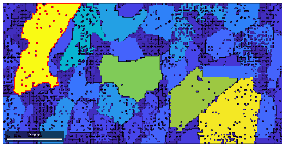
Note that this way of addressing individual grains can be generalized to many grains. E.g. assume we are interested in the largest 5 grains. Then we can sort the vector grain_area and take the indices of the 5 largest grains.
[sorted_area,sorted_id] = sort(grain_area,'descend');

large_grain_id = sorted_id(1:5);

hold on
plot(grains(large_grain_id).boundary,'linecolor','green','linewidth',1.5)
hold off
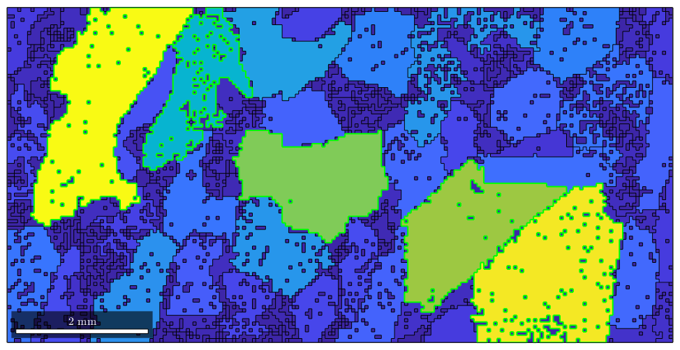
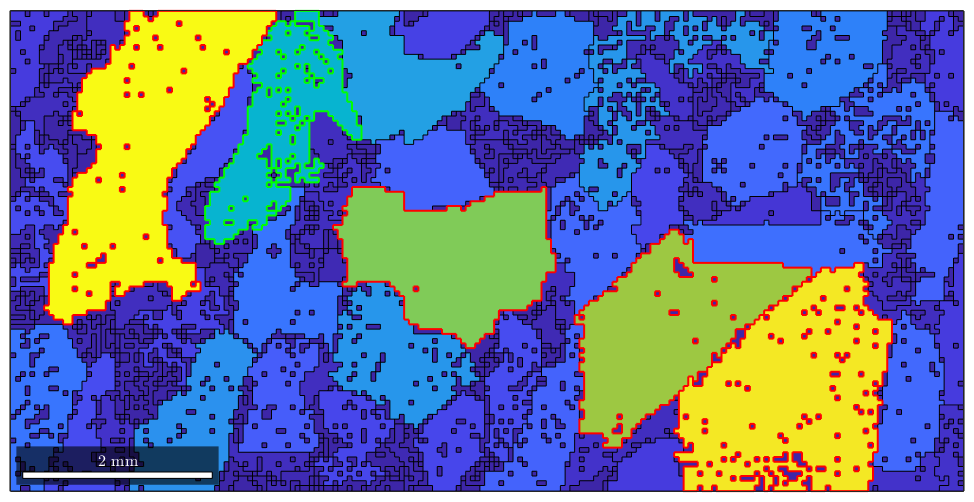
Indexing by a Condition
By the same syntax as above we can also single out grains that satisfy a certain condition. I.e., to access are grains that are at least half as large as the largest grain we can do
condition = grain_area > max_area/2;

hold on
plot(grains(condition).boundary,'linecolor','red','linewidth',1.5)
hold off
This is a very powerful way of accessing grains as the condition can be build up using any grain property. As an example let us consider the phase. The phase of the first five grains we get by
grains(1:5).phase
ans =
     0
     0
     0
     0
     2
Now we can access or grains of the first phase Forsterite by the condition
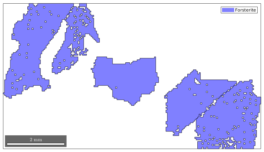
condition = grains.phase == 1;
plot(grains(condition))
To make the above more directly you can use the mineral name for indexing
grains('forsterite')
ans = grain2d

 Phase  Grains  Pixels     Mineral  Symmetry  Crystal reference frame
     1     242   14093  Forsterite       mmm

 boundary segments: 7670
 triple points: 795

 Properties: GOS, meanRotation
Logical indexing allows also for more complex queries, e.g. selecting all grains perimeter larger than 6000 and at least 600 measurements within
condition = grains.perimeter>6000 & grains.grainSize >= 600;

selected_grains = grains(condition)

plot(selected_grains)
selected_grains = grain2d

 Phase  Grains  Pixels     Mineral  Symmetry  Crystal reference frame
     1       5    5784  Forsterite       mmm

 boundary segments: 1893
 triple points: 244

   Id   Phase   Pixels          GOS   phi1   Phi   phi2
  798       1     1447     0.013232    166   127    259
  876       1     1075   0.00805971    153    68    237
  999       1     1044   0.00753116     89    99    224
 1617       1     1548    0.0129383    167    81    251
 1620       1      670    0.0870135    143    78    274
Indexing by orientation or position
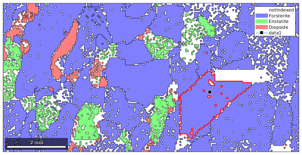
One can also select a grain by its spatial coordinates using the syntax grains(x,y)
x = 12000; y = 4000;

plot(grains);

hold on

plot(grains(x,y).boundary,'linewidth',2,'linecolor','r')

plot(x,y,'marker','s','markerfacecolor','k',...
  'markersize',10,'markeredgecolor','w')
hold off
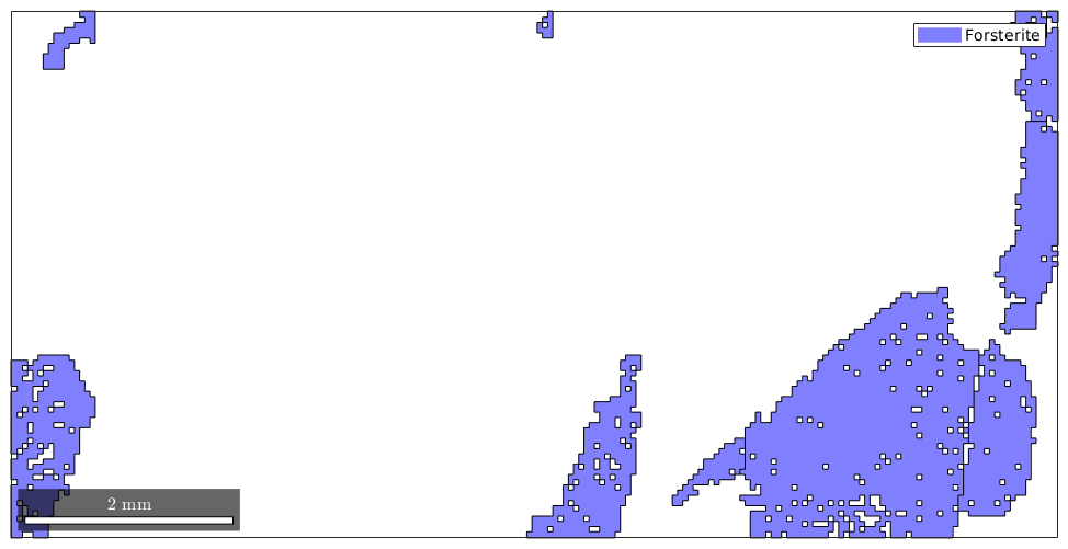
In order to select all grains with a certain orientation one can do
% restrict first to Forsterite phase
grains_fo = grains('fo')

% the reference orientation
ori = orientation.byEuler(350*degree,50*degree,100*degree,grains('fo').CS)

% select all grain with misorientation angle to ori less then 20 degree
grains_selected = grains_fo(angle(grains_fo.meanOrientation,ori)<20*degree)

plot(grains_selected)
grains_fo = grain2d

 Phase  Grains  Pixels     Mineral  Symmetry  Crystal reference frame
     1     242   14093  Forsterite       mmm

 boundary segments: 7670
 triple points: 795

 Properties: GOS, meanRotation


ori = orientation
  size: 1 x 1
  crystal symmetry : Forsterite (mmm)
  specimen symmetry: 1

  Bunge Euler angles in degree
  phi1  Phi phi2 Inv.
   350   50  100    0


grains_selected = grain2d

 Phase  Grains  Pixels     Mineral  Symmetry  Crystal reference frame
     1      12    2979  Forsterite       mmm

 boundary segments: 1603
 triple points: 173

   Id   Phase   Pixels          GOS   phi1   Phi   phi2
  359       1       63    0.0129176    177   140    250
  389       1        1            0    167   128    260
  622       1      352   0.00896432    153   122    252
  636       1      305    0.0156453    164   115    268
  680       1      331    0.0198713    152   143    247
  798       1     1447     0.013232    166   127    259
 1297       1      289    0.0315393    166   147    260
 1549       1        1            0      1    47    279
 1609       1       48    0.0169152    158   139    259
 1629       1       10    0.0193004    172   125    261
 1660       1      129   0.00814837      1    47    279
 1662       1        3   0.00475795      1    47    279
Grain-size Analysis
Let's go back to the grain size and analyze its distribution. To this end, we consider the complete data set.
mtexdata forsterite
% consider only indexed data for grain segmentation
ebsd = ebsd('indexed');
% perform grain segmentation
[grains,ebsd.grainId] = calcGrains(ebsd)
grains = grain2d

 Phase  Grains  Pixels     Mineral  Symmetry  Crystal reference frame
     1    1080  152345  Forsterite       mmm
     2     515   26058   Enstatite       mmm
     3    1496    9064    Diopside     12/m1       X||a*, Y||b*, Z||c

 boundary segments: 43912
 triple points: 3417

 Properties: GOS, meanRotation


ebsd = EBSD

 Phase  Orientations     Mineral        Color  Symmetry  Crystal reference frame
     1  152345 (81%)  Forsterite   light blue       mmm
     2   26058 (14%)   Enstatite  light green       mmm
     3   9064 (4.8%)    Diopside    light red     12/m1       X||a*, Y||b*, Z||c

 Properties: bands, bc, bs, error, mad, x, y, grainId
 Scan unit : um
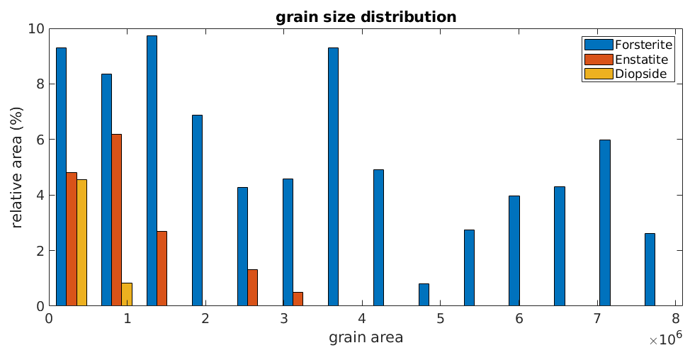
Then the following command gives you a nice overview over the grain size distributions of the grains
hist(grains)
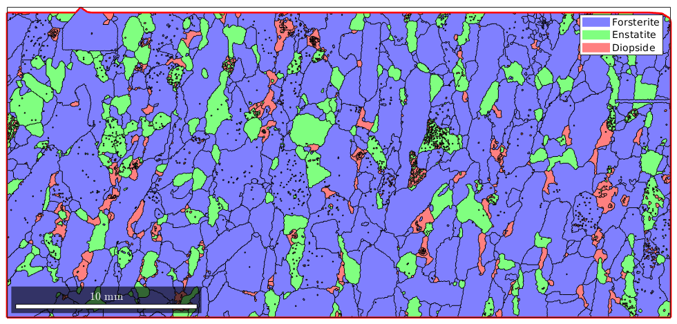
Sometimes it is desirable to remove all boundary grains as they might distort grain statistics. To do so one should remember that each grain boundary has a property grainId which stores the ids of the neigbouring grains. In the case of an outer grain boundary, one of the neighbouring grains has the id zero. We can filter out all these boundary segments by
% ids of the outer boundary segment
outerBoundary_id = any(grains.boundary.grainId==0,2);

plot(grains)
hold on
plot(grains.boundary(outerBoundary_id),'linecolor','red','linewidth',2)
hold off
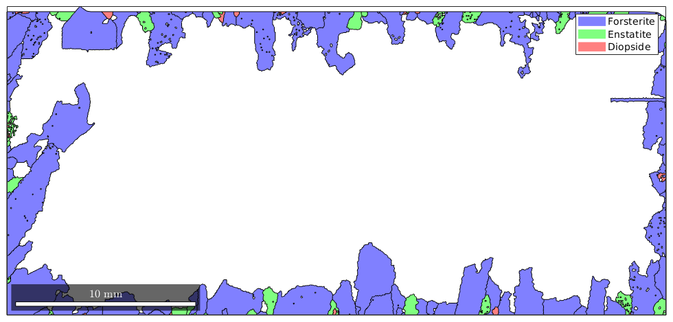
Now grains.boundary(outerBoundary_id).grainId is a list of grain ids where the first column is zero, indicating the outer boundary, and the second column contains the id of the boundary grain. Hence, it remains to remove all grains with these ids.
% next we compute the corresponding grain_id
grain_id = grains.boundary(outerBoundary_id).grainId;

% remove all zeros
grain_id(grain_id==0) = [];

% and plot the boundary grains
plot(grains(grain_id))
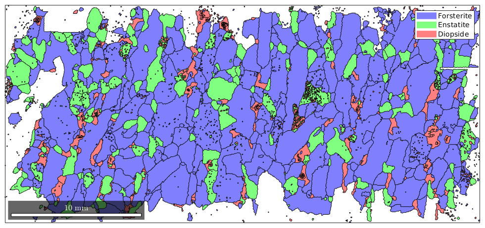
finally, we can remove the boundary grains by
grains(grain_id) = []

plot(grains)
grains = grain2d

 Phase  Grains  Pixels     Mineral  Symmetry  Crystal reference frame
     1     968  116882  Forsterite       mmm
     2     480   23877   Enstatite       mmm
     3    1467    8871    Diopside     12/m1       X||a*, Y||b*, Z||c

 boundary segments: 40105
 triple points: 3383

 Properties: GOS, meanRotation
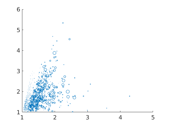
Beside the area, there are various other geometric properties that can be computed for grains, e.g., the perimeter, the diameter, the equivalentRadius, the equivalentPerimeter, the aspectRatio, and the shapeFactor. The following is a simple scatter plot of shape factor against aspect ratio to check for correlation.
% the size of the dots corresponds to the area of the grains
close all
scatter(grains.shapeFactor, grains.aspectRatio, 70*grains.area./max(grains.area))
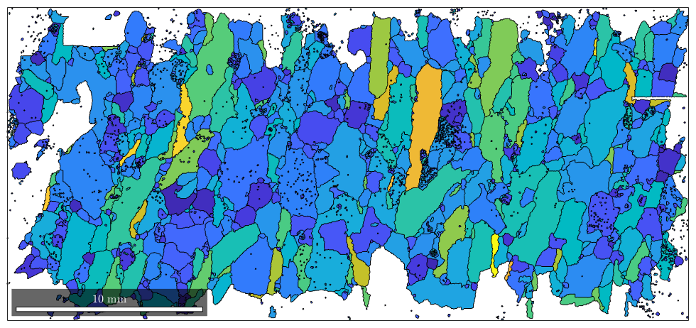
plot(grains,log(grains.aspectRatio))
Spatial Dependencies
One interesting question would be, whether a polyphase system has dependence in the spatial arrangement or not, therefore, we can count the transitions to a neighbour grain
%[J, T, p ] = joinCount(grains,grains.phase)
| DocHelp 0.1 beta |