Plotting grains
how to colorize grains
| On this page ... |
| Phase maps |
| Orientation Maps |
| Plotting arbitrary properties |
| Colorizing circular properties |
| Plotting the orientation within a grain |
| Visualizing directions |
| Labeling Grains |
We start by importing some EBSD data and reconstructing some grains
% import a demo data set
mtexdata forsterite
plotx2east

% consider only indexed data for grain segmentation
ebsd = ebsd('indexed');

% perform grain segmentation
[grains,ebsd.grainId,ebsd.mis2mean] = calcGrains(ebsd);
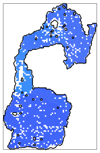
Phase maps
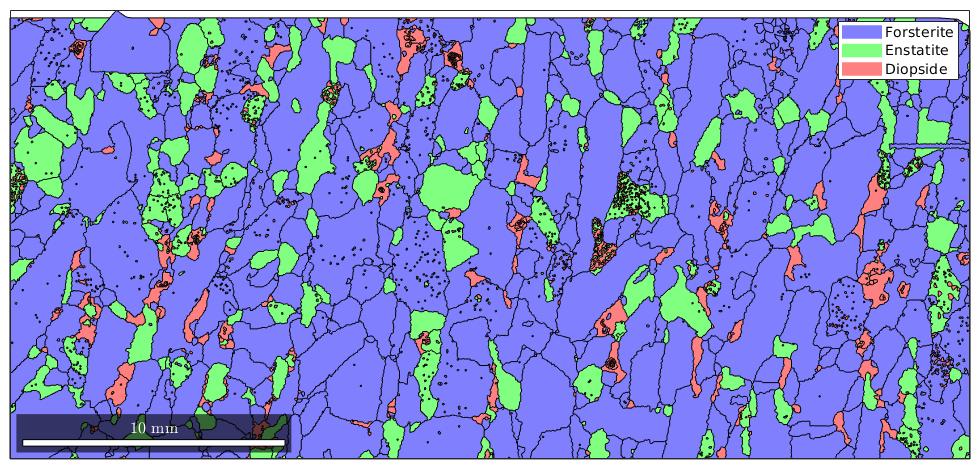
When using the plot command without additional argument the associated color is defined by color stored in the crystal symmetry for each phase
close all
plot(grains)

grains('Fo').CS.color
ans =
    'light blue'
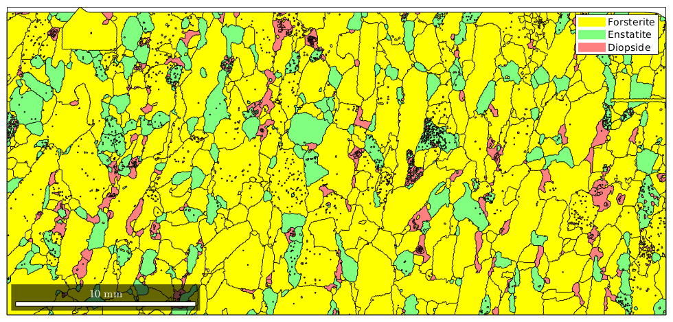
Accodingly, changing the color stored in the crystal symmetry changes the color in the map
grains('Fo').CS.color = 'yellow'
plot(grains)
grains = grain2d

 Phase  Grains  Pixels     Mineral  Symmetry  Crystal reference frame
     1    1080  152345  Forsterite       mmm
     2     515   26058   Enstatite       mmm
     3    1496    9064    Diopside     12/m1       X||a*, Y||b*, Z||c

 boundary segments: 43912
 triple points: 3417

 Properties: GOS, meanRotation
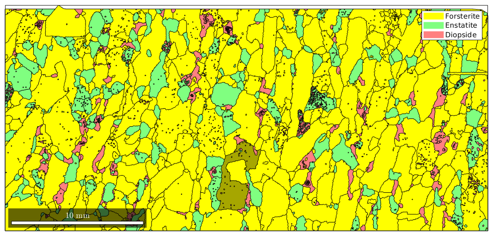
The color can also been specified directly by using the option FaceColor. Note, that this requires the color to be specified by RGB values.
% detect the largest grain
[~,id] = max(grains.area);

% plot the grain in black with some transperency
hold on
plot(grains(id),'FaceColor',[0 0 0],'FaceAlpha',0.35)
hold off
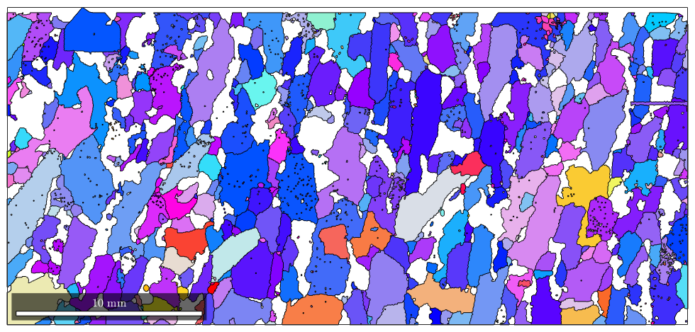
Orientation Maps
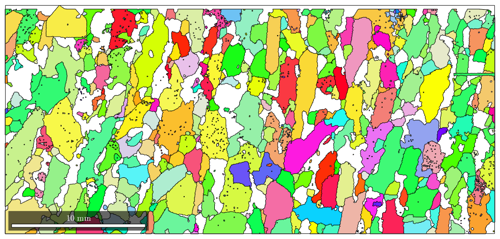
Coloring grains according to their mean orientations is very similar to EBSD maps colored by orientations. The most important thing is that the misorientation can only extracte from grains of the same phase.
% the implicite way
plot(grains('Fo'),grains('fo').meanOrientation)
  I'm going to colorize the orientation data with the
  standard MTEX colorkey. To view the colorkey do:

  colorKey = ipfColorKey(ori_variable_name)
  plot(colorKey)
This implicte way gives no control about how the color is computed from the meanorientation. When using the explicite way by defining a orientation to color map
% this defines a ipf color key
ipfKey = ipfColorKey(grains('Fo'));
we can set the inverse pole figure direction and many other properties
ipfKey.inversePoleFigureDirection = xvector;

% compute the colors from the meanorientations
color = ipfKey.orientation2color(grains('Fo').meanOrientation);

% and use them for plotting
plot(grains('fo'),color)
Plotting arbitrary properties
As we have seen in the previous section the plot command accepts as second argument any list of RGB values specifying a color. Instead of RGB values the second argument can also be a list of values which are then transformed by a colormap into color.
As an example we colorize the grains according to their aspect ratio.
plot(grains,grains.aspectRatio)
we see that we have a very alongated grain which makes it difficult to distinguesh the aspect ration of the other grains. A solution for this is to specify the values of the aspect ration which should maped to the top and bottom color of the colormap
CLim(gcm,[1 5])
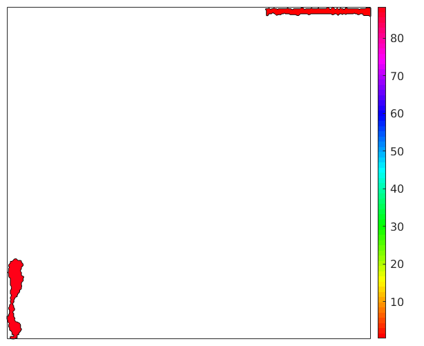
Colorizing circular properties
Sometimes the property we want to display is a circular, e.g., the direction of the grain alongation. In this case it is important to use a circular colormap which assign the same color to high values and low values. In the case of the direction of the grain alongation the angles 0 and 180 should get the same color since they represent the same direction.
% consider only alongated grains
alongated_grains = grains(grains.aspectRatio > 5);

% get the grain alongation
dir = alongated_grains.principalComponents;

% transfer this into degree and project it into the interval [0,180]
dir = mod(dir./degree,180);

% plot the direction
plot(alongated_grains,dir,'micronbar','off')

% change the default colormap to a circular one
mtexColorMap HSV

% display the colormap
mtexColorbar
Plotting the orientation within a grain
In order to plot the orientations of EBSD data within certain grains one first has to extract the EBSD data that belong to the specific grains.
% let have a look at the bigest grain
[~,id] = max(grains.area)

% and select the corresponding EBSD data
ebsd_maxGrain = ebsd(ebsd.grainId == id)

% the previous command is equivalent to the more simpler
ebsd_maxGrain = ebsd(grains(id));
id =
   931

ebsd_maxGrain = EBSD

 Phase  Orientations     Mineral       Color  Symmetry  Crystal reference frame
     1   2683 (100%)  Forsterite  light blue       mmm

 Properties: bands, bc, bs, error, mad, x, y, grainId, mis2mean
 Scan unit : um
% compute the color out of the orientations
color = ipfKey.orientation2color(ebsd_maxGrain.orientations);

% plot it
plot(ebsd_maxGrain, color,'micronbar','off')

% plot the grain boundary on top
hold on
plot(grains(id).boundary,'linewidth',2)
hold off
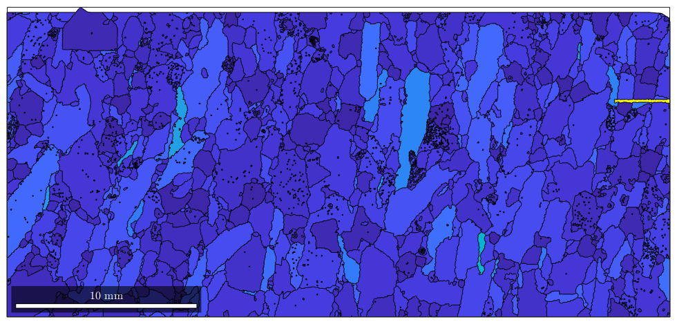
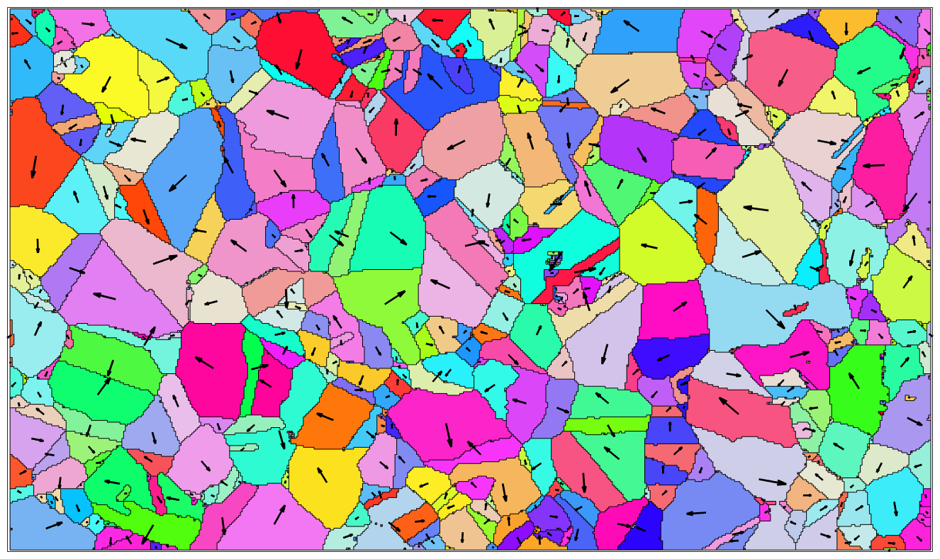
Visualizing directions
We may also visualize directions by arrows placed at the center of the grains.
% load some single phase data set
mtexdata csl

% compute and plot grains
[grains,ebsd.grainId] = calcGrains(ebsd);
plot(grains,grains.meanOrientation,'micronbar','off','figSize','large')

% next we want to visualize the direction of the 100 axis
dir = grains.meanOrientation * Miller(1,0,0,grains.CS);

% the lenght of the vectors should depend on the grain diameter
len = 0.25*grains.diameter;

% arrows are plotted using the command quiver. We need to switch of auto
% scaling of the arrow length
hold on
quiver(grains,len.*dir,'autoScale','off','color','black')
hold off
  I'm going to colorize the orientation data with the
  standard MTEX colorkey. To view the colorkey do:

  colorKey = ipfColorKey(ori_variable_name)
  plot(colorKey)
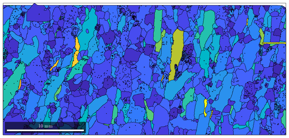
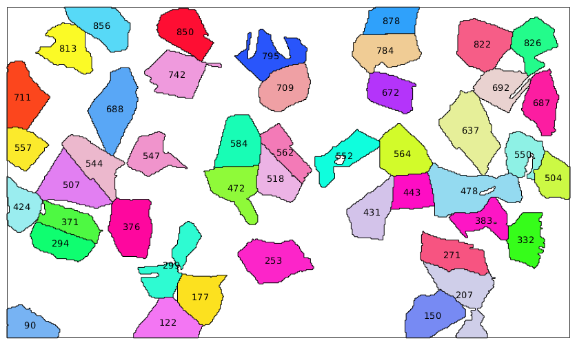
Labeling Grains
In the above example the vectors are centered at the centroids of the grains. Other elements
% only the very big grains
big_grains = grains(grains.grainSize>1000);

% plot them
plot(big_grains,big_grains.meanOrientation,'micronbar','off')

% plot on top their ids
text(big_grains,int2str(big_grains.id))
  I'm going to colorize the orientation data with the
  standard MTEX colorkey. To view the colorkey do:

  colorKey = ipfColorKey(ori_variable_name)
  plot(colorKey)
| DocHelp 0.1 beta |