Analyzing Individual Grains
how to work with single grains
| On this page ... |
| Connection between grains and EBSD data |
| Visualize the misorientation within a grain |
| Testing on Bingham distribution for a single grain |
| Profiles through a single grain |
Connection between grains and EBSD data
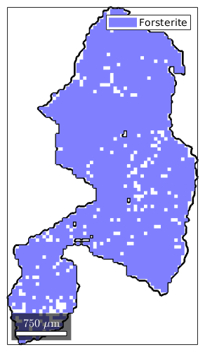
As usual, we start by importing some EBSD data and computing grains
close all
mtexdata forsterite
plotx2east

% consider only indexed data for grain segmentation
ebsd = ebsd('indexed');

% compute the grains
[grains,ebsd.grainId,ebsd.mis2mean] = calcGrains(ebsd);
The grains contain. We can access these data by
grain_selected = grains( grains.grainSize >=  1160)
ebsd_selected = ebsd(grain_selected)
grain_selected = grain2d

 Phase  Grains  Pixels     Mineral  Symmetry  Crystal reference frame
     1      32   62262  Forsterite       mmm

 boundary segments: 11070
 triple points: 782

 Properties: GOS, meanRotation


ebsd_selected = EBSD

 Phase  Orientations     Mineral       Color  Symmetry  Crystal reference frame
     1  62262 (100%)  Forsterite  light blue       mmm

 Properties: bands, bc, bs, error, mad, x, y, grainId, mis2mean
 Scan unit : um
A more convenient way to select grains in daily practice is by spatial coordinates.
grain_selected = grains(12000,3000)
grain_selected = grain2d

 Phase  Grains  Pixels     Mineral  Symmetry  Crystal reference frame
     1       1    1208  Forsterite       mmm

 boundary segments: 238
 triple points: 18

  Id   Phase   Pixels          GOS   phi1   Phi   phi2
 640       1     1208   0.00806772    153    68    237
you can get the id of this grain by
grain_selected.id
ans =
   640
let's look for the grain with the largest grain orientation spread
[~,id] = max(grains.GOS)
grain_selected = grains(id)
id =
        1856

grain_selected = grain2d

 Phase  Grains  Pixels     Mineral  Symmetry  Crystal reference frame
     1       1    2614  Forsterite       mmm

 boundary segments: 458
 triple points: 28

   Id   Phase   Pixels        GOS   phi1   Phi   phi2
 1856       1     2614   0.170662    153   109    247
plot(grain_selected.boundary,'linewidth',2)
hold on
plot(ebsd(grain_selected))
hold off
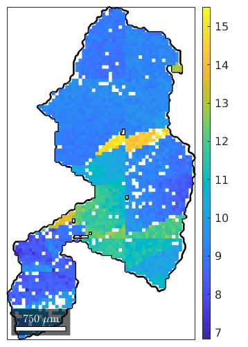
Visualize the misorientation within a grain
close
plot(grain_selected.boundary,'linewidth',2)
hold on
plot(ebsd(grain_selected),ebsd(grain_selected).mis2mean.angle./degree)
hold off
mtexColorbar
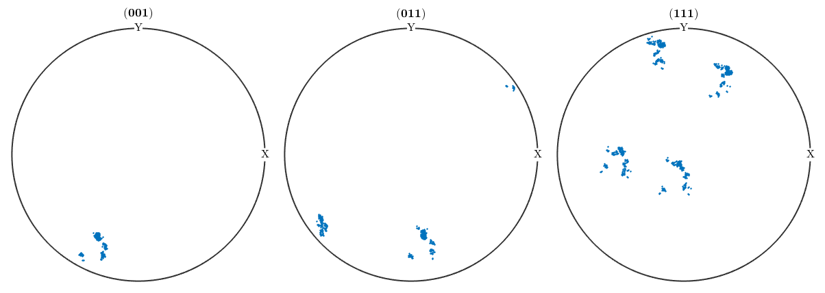
Testing on Bingham distribution for a single grain
Although the orientations of an individual grain are highly concentrated, they may vary in the shape. In particular, if the grain was deformed by some process, we are interested in quantifications.
cs = ebsd(grain_selected).CS;
ori = ebsd(grain_selected).orientations;
plotPDF(ori,[Miller(0,0,1,cs),Miller(0,1,1,cs),Miller(1,1,1,cs)],'antipodal')
I'm plotting 1250 random orientations out of 2614 given orientations You can specify the the number points by the option "points". The option "all" ensures that all data are plotted
Testing on the distribution shows a gentle prolatness, nevertheless we would reject the hypothesis for some level of significance, since the distribution is highly concentrated and the numerical results vague.
calcBinghamODF(ori,'approximated')
ans = ODF
  crystal symmetry : Forsterite (mmm)
  specimen symmetry: 1

  Bingham portion:
     kappa: 0 4019.3061 4021.4833 4022.7958
    weight: 1
T_spherical = bingham_test(ori,'spherical','approximated');
T_prolate   = bingham_test(ori,'prolate',  'approximated');
T_oblate    = bingham_test(ori,'oblate',   'approximated');

[T_spherical T_prolate T_oblate]
ans =
     1     1     1
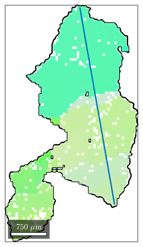
Profiles through a single grain
Sometimes, grains show large orientation difference when being deformed and then its of interest, to characterize the lattice rotation. One way is to order orientations along certain line segment and look at the profile.
We proceed by specifying such a line segment
close,   plot(grain_selected.boundary,'linewidth',2)
hold on, plot(ebsd(grain_selected),ebsd(grain_selected).orientations)

% line segment
lineSec =  [18826   6438; 18089 10599];

line(lineSec(:,1),lineSec(:,2),'linewidth',2)
The command spatialProfile restricts the EBSD data to this line
ebsd_line = spatialProfile(ebsd(grain_selected),lineSec);
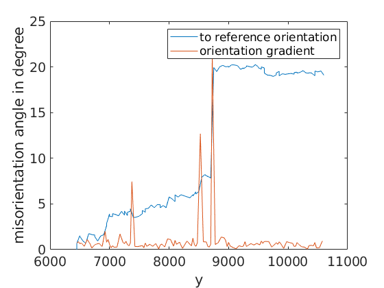
Next, we plot the misorientation angle to the first point of the line as well as the orientation gradient
close all % close previous plots

% misorientation angle to the first orientation on the line
plot(ebsd_line.y,...
  angle(ebsd_line(1).orientations,ebsd_line.orientations)/degree)

% misorientation gradient
hold all
plot(0.5*(ebsd_line.y(1:end-1)+ebsd_line.y(2:end)),...
  angle(ebsd_line(1:end-1).orientations,ebsd_line(2:end).orientations)/degree)
hold off

xlabel('y'); ylabel('misorientation angle in degree')

legend('to reference orientation','orientation gradient')
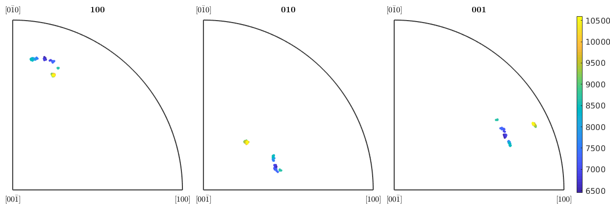
We can also plot the orientations along this line into inverse pole figures and colorize them according to their y-coordinate
close, plotIPDF(ebsd_line.orientations,[xvector,yvector,zvector],...
  'property',ebsd_line.y,'markersize',3,'antipodal')

mtexColorbar
| DocHelp 0.1 beta |