Grain Reconstruction
Grain Reconstruction from EBSD data.
Let us first import some example EBSD data and restrict it to a subregion of interest.
close all; plotx2east
mtexdata forsterite
ebsd = ebsd(inpolygon(ebsd,[5 2 10 5]*10^3));
plot(ebsd)
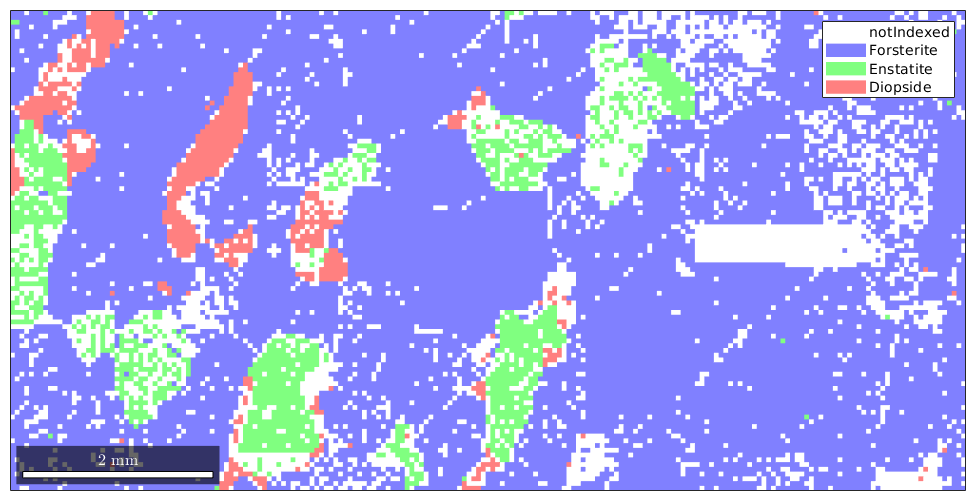
Basic grain reconstruction
We see that there are a lot of not indexed measurements. For grain reconstruction, we have three different choices how to deal with these unindexed regions:
- leaf them unindexed
- assign them to the surrounding grains
- a mixture of both, e.g., assign small notindexed regions to the surrounding grains but keep large notindexed regions
By default, MTEX uses the first method.
The second parameter that is involved in grain reconstruction is the threshold misorientation angle indicating a grain boundary. By default, this value is set to 10 degrees.
All grain reconstruction methods in MTEX are accessible via the command calcGrains which takes as input an EBSD data set and returns a list of grain.
grains = calcGrains(ebsd,'angle',10*degree)
grains = grain2d

 Phase  Grains  Pixels     Mineral  Symmetry  Crystal reference frame
     0    1139    4052  notIndexed
     1     244   14093  Forsterite       mmm
     2     177    1397   Enstatite       mmm
     3     104     759    Diopside     12/m1       X||a*, Y||b*, Z||c

 boundary segments: 10422
 triple points: 905

 Properties: GOS, meanRotation
The reconstructed grains are stored in the variable grains. Note that also the notIndexed measurements are grouped into grains. This allows later to analyze the shape of these unindexed regions.
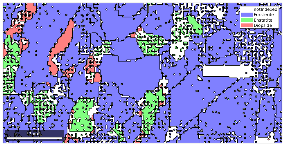
To visualize the grains we can plot its boundaries by the command plotBoundary.
% start overide mode
hold on

% plot the boundary of all grains
plot(grains.boundary,'linewidth',1.5)

% stop overide mode
hold off
The grainId and how to select EBSD inside specific grains
Besides, the list of grains the command calcGrains returns also two other output arguments.
[grains,ebsd.grainId,ebsd.mis2mean] = calcGrains(ebsd,'angle',7.5*degree);
grains
ebsd
grains = grain2d

 Phase  Grains  Pixels     Mineral  Symmetry  Crystal reference frame
     0    1139    4052  notIndexed
     1     245   14093  Forsterite       mmm
     2     177    1397   Enstatite       mmm
     3     105     759    Diopside     12/m1       X||a*, Y||b*, Z||c

 boundary segments: 10430
 triple points: 911

 Properties: GOS, meanRotation


ebsd = EBSD

 Phase  Orientations     Mineral        Color  Symmetry  Crystal reference frame
     0    4052 (20%)  notIndexed
     1   14093 (69%)  Forsterite   light blue       mmm
     2   1397 (6.9%)   Enstatite  light green       mmm
     3    759 (3.7%)    Diopside    light red     12/m1       X||a*, Y||b*, Z||c

 Properties: bands, bc, bs, error, mad, x, y, grainId, mis2mean
 Scan unit : um
The second output argument grainId is a list with the same size as the EBSD measurements that stores for each measurement the corresponding grainId. The above syntax stores this list directly inside the ebsd variable. This enables MTEX to select EBSD data by grains. The following command returns all the EBSD data that belong to grain number 33.
ebsd(grains(33))
ans = EBSD

 Phase  Orientations   Mineral      Color  Symmetry  Crystal reference frame
     3      5 (100%)  Diopside  light red     12/m1       X||a*, Y||b*, Z||c

    Id   Phase   phi1   Phi   phi2   bands    bc    bs   error   mad      x      y   grainId   phi1   Phi   phi2
 29476       3    170    80     42       7   140   255       0     1   9750   2000        33     38     0    322
 29477       3    171    80     42       7   137   234       0     1   9800   2000        33    173     1    187
 29478       3    171    79     41       7   152   245       0   1.1   9850   2000        33    302     1     59
 29479       3    170    81     42       7   105   153       0   0.8   9900   2000        33    122     2    239
 30208       3    170    79     42       7   110   211       0   0.8   9750   2050        33    341     1     20
 Scan unit : um
and is equivalent to the command
ebsd(ebsd.grainId == 33)
ans = EBSD

 Phase  Orientations   Mineral      Color  Symmetry  Crystal reference frame
     3      5 (100%)  Diopside  light red     12/m1       X||a*, Y||b*, Z||c

    Id   Phase   phi1   Phi   phi2   bands    bc    bs   error   mad      x      y   grainId   phi1   Phi   phi2
 29476       3    170    80     42       7   140   255       0     1   9750   2000        33     38     0    322
 29477       3    171    80     42       7   137   234       0     1   9800   2000        33    173     1    187
 29478       3    171    79     41       7   152   245       0   1.1   9850   2000        33    302     1     59
 29479       3    170    81     42       7   105   153       0   0.8   9900   2000        33    122     2    239
 30208       3    170    79     42       7   110   211       0   0.8   9750   2050        33    341     1     20
 Scan unit : um
Misorientation to mean orientation
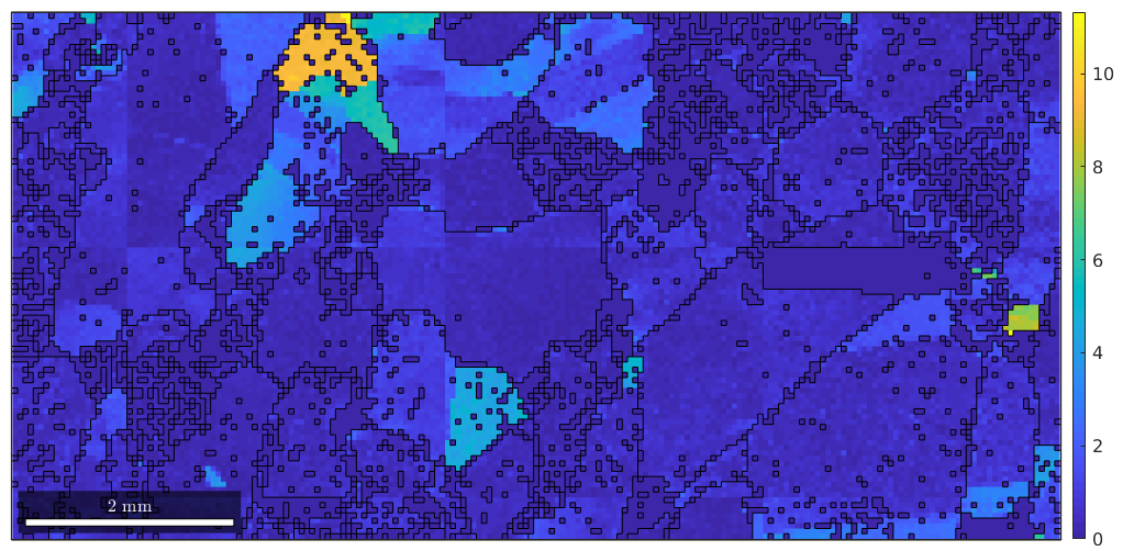
The third output argument is again a list of the same size as the ebsd measurements. The entries are the misorientation to the mean orientation of the corresponding grain.
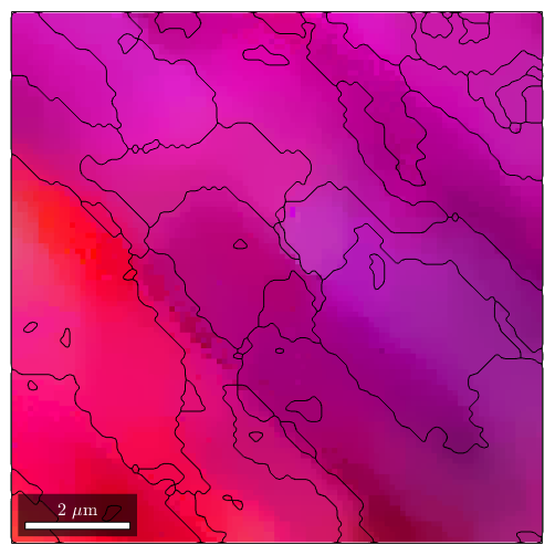
plot(ebsd,ebsd.mis2mean.angle ./ degree)

hold on
plot(grains.boundary)
hold off

mtexColorbar
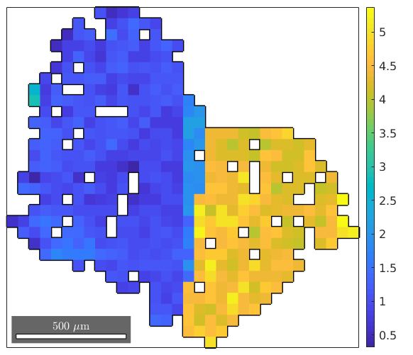
We can examine the misorientation to mean for one specific grain as follows
% select a grain by coordinates
myGrain = grains(9075,3275)
plot(myGrain.boundary,'linewidth',2)

% plot mis2mean angle for this specific grain
hold on
plot(ebsd(myGrain),ebsd(myGrain).mis2mean.angle ./ degree)
hold off
mtexColorbar
myGrain = grain2d

 Phase  Grains  Pixels     Mineral  Symmetry  Crystal reference frame
     1       1     497  Forsterite       mmm

 boundary segments: 294
 triple points: 32

  Id   Phase   Pixels         GOS   phi1   Phi   phi2
 762       1      497   0.0400864    131    64    249
Filling notindexed holes
It is important to understand that MTEX distinguishes the following two situations
- a location is marked as notindexed
- a location does not occur in the data set
A location marked as notindexed is interpreted by MTEX as at this position, there is no crystal, whereas for a location that does not occur in the data set is interpreted by MTEX as: it is not known whether there is a crystal or not. Just to remind you, the later assumption is nothing special as it applies at all locations but the measurement points.
A location that does not occur in the data is assigned in MTEX to the same grain and phase as the closest measurement point - this may also be a notindexed point. Hence, filling holes in MTEX means to erase them from the list of measurements, i.e., instead of telling MTEX there is no crystal we are telling MTEX: we do not know what there is.
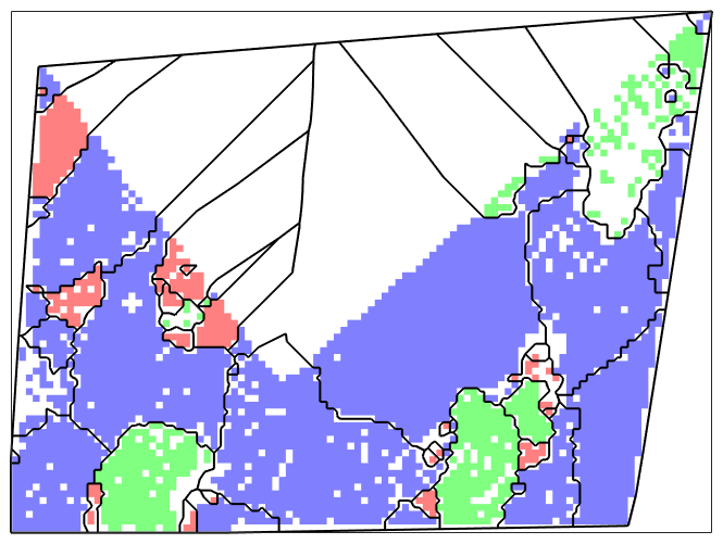
The extremal case is to say whenever there is a not indexed measurement we actually do not know anything and allow MTEX to freely guess what happens there. This is realized by removing all not indexed measurements or, equivalently, computing the grains only from the indexed measurements
% compute the grains from the indexed measurements only
grains = calcGrains(ebsd('indexed'))

plot(ebsd)

% start overide mode
hold on

% plot the boundary of all grains
plot(grains.boundary,'linewidth',1.5)

% mark two grains by location
plot(grains(11300,6100).boundary,'linecolor','m','linewidth',2,...
  'DisplayName','grain A')
plot(grains(12000,4000).boundary,'linecolor','r','linewidth',2,...
  'DisplayName','grain B')

% stop overide mode
hold off
grains = grain2d

 Phase  Grains  Pixels     Mineral  Symmetry  Crystal reference frame
     1     103   14093  Forsterite       mmm
     2      32    1397   Enstatite       mmm
     3      71     759    Diopside     12/m1       X||a*, Y||b*, Z||c

 boundary segments: 3784
 triple points: 240

 Properties: GOS, meanRotation
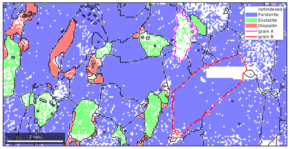
We observe, especially in the marked grains, how MTEX fills notindexed regions and connects otherwise separate measurements to grains. As all information about not indexed regions were removed the reconstructed grains fill the map completely
plot(grains,'linewidth',2)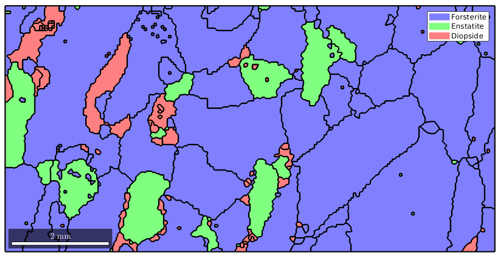
Inside of grain B, there is a large not indexed region and we might argue that is not very meaningful to assign such a large region to some grain but should have kept it not indexed. In order to decide which not indexed region is large enough to be kept not indexed and which not indexed regions can be filled it is helpful to know that the command calcGrains also separates the not indexed regions into "grains" and we can standard grain functions like area or perimeter to analyze these regions.
[grains,ebsd.grainId,ebsd.mis2mean] = calcGrains(ebsd);
notIndexed = grains('notIndexed')
notIndexed = grain2d

 Phase  Grains  Pixels     Mineral  Symmetry  Crystal reference frame
     0    1139    4052  notIndexed

 boundary segments: 8694
 triple points: 868

 Properties: GOS, meanRotation
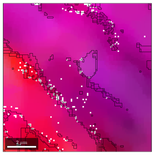
We see that we have 1139 not indexed regions. A good measure for compact regions vs. cluttered regions is the quotient between the area and the boundary length.
% plot the not indexed regions colorcoded according the the quotient between
% number of measurements and number of boundary segments
plot(notIndexed,log(notIndexed.grainSize ./ notIndexed.boundarySize))
mtexColorbar
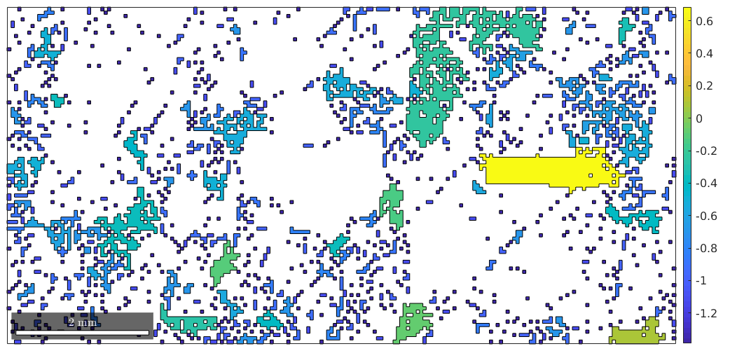
Regions with a high quotient are blocks which can be hardly correctly assigned to a grain. Hence, we should keep these regions as not indexed and only remove the not indexed information from locations with a low quotient.
% the "not indexed grains" we want to remove
toRemove = notIndexed(notIndexed.grainSize ./ notIndexed.boundarySize<0.8)

% now we remove the corresponding EBSD measurements
ebsd(toRemove) = []

% and perform grain reconstruction with the reduces EBSD data set
[grains,ebsd.grainId,ebsd.mis2mean] = calcGrains(ebsd);

plot(grains)
toRemove = grain2d

 Phase  Grains  Pixels     Mineral  Symmetry  Crystal reference frame
     0    1134    3442  notIndexed

 boundary segments: 8256
 triple points: 837

 Properties: GOS, meanRotation


ebsd = EBSD

 Phase  Orientations     Mineral        Color  Symmetry  Crystal reference frame
     0    610 (3.6%)  notIndexed
     1   14093 (84%)  Forsterite   light blue       mmm
     2   1397 (8.3%)   Enstatite  light green       mmm
     3    759 (4.5%)    Diopside    light red     12/m1       X||a*, Y||b*, Z||c

 Properties: bands, bc, bs, error, mad, x, y, grainId, mis2mean
 Scan unit : um
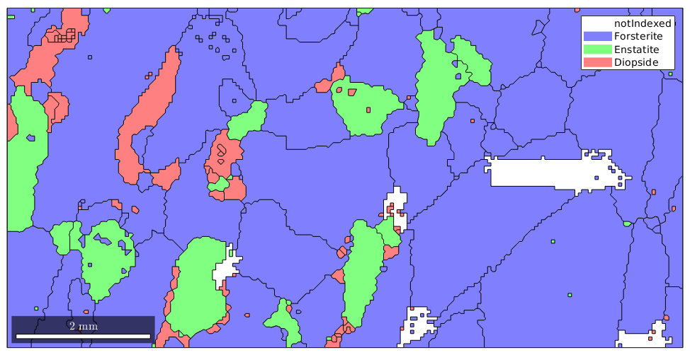
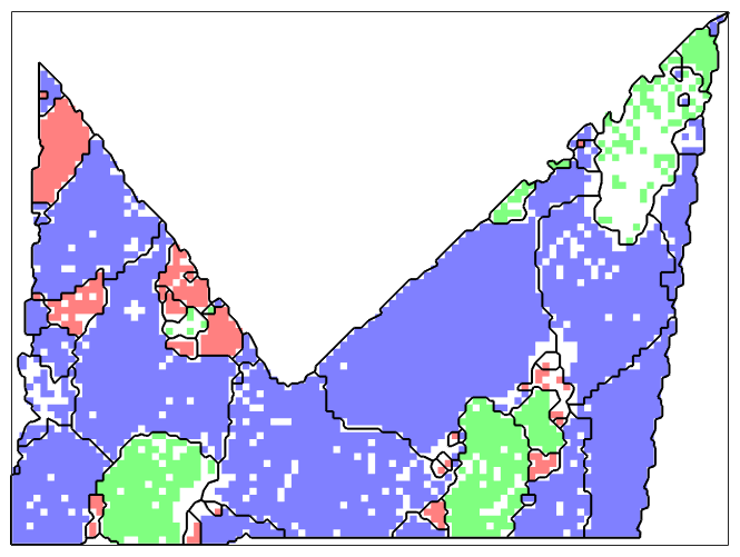
We see that there are some, not indexed regions are left blank. Finally, the image with the raw EBSD data and on top the grain boundaries.
% plot the raw data
plot(ebsd)

% start overide mode
hold on

% plot the boundary of all grains
plot(grains.boundary,'linewidth',1.5)

% mark two grains by location
plot(grains(11300,6100).boundary,'linecolor','m','linewidth',2,...
  'DisplayName','grain A')
plot(grains(12000,4000).boundary,'linecolor','r','linewidth',2,...
  'DisplayName','grain B')

% stop overide mode
hold off

Non convex data sets
By default MTEX uses the convex hull when computing the outer boundary for an EBSD data set. This leads to poor results in the case of non convex EBSD data sets
% cut of a non convex region from our previous data set
poly = 1.0e+04 *[...
  0.6853    0.2848
  0.7102    0.6245
  0.8847    0.3908
  1.1963    0.6650
  1.1371    0.2880
  0.6853    0.2833
  0.6853    0.2848];

ebsdP = ebsd(ebsd.inpolygon(poly))

plot(ebsdP,'micronBar','off')
legend off

% compute the grains
grains = calcGrains(ebsdP('indexed'))

% plot the grain boundary
hold on
plot(grains.boundary,'linewidth',1.5)
hold off
ebsdP = EBSD

 Phase  Orientations     Mineral        Color  Symmetry  Crystal reference frame
     0      107 (3%)  notIndexed
     1    2756 (78%)  Forsterite   light blue       mmm
     2     452 (13%)   Enstatite  light green       mmm
     3    231 (6.5%)    Diopside    light red     12/m1       X||a*, Y||b*, Z||c

 Properties: bands, bc, bs, error, mad, x, y, grainId, mis2mean
 Scan unit : um


grains = grain2d

 Phase  Grains  Pixels     Mineral  Symmetry  Crystal reference frame
     1      26    2756  Forsterite       mmm
     2       8     452   Enstatite       mmm
     3      22     231    Diopside     12/m1       X||a*, Y||b*, Z||c

 boundary segments: 1024
 triple points: 66

 Properties: GOS, meanRotation
We see that the grains badly fill up the entire convex hull of the data points. This can be avoided by specifying the option tight for the determination of the outer boundary.
plot(ebsdP,'micronBar','off')
legend off

% compute the grains
grains = calcGrains(ebsdP('indexed'),'boundary','tight')

% plot the grain boundary
hold on
plot(grains.boundary,'linewidth',1.5)
hold off
grains = grain2d

 Phase  Grains  Pixels     Mineral  Symmetry  Crystal reference frame
     1      28    2756  Forsterite       mmm
     2       9     452   Enstatite       mmm
     3      22     231    Diopside     12/m1       X||a*, Y||b*, Z||c

 boundary segments: 1252
 triple points: 61

 Properties: GOS, meanRotation
Grain smoothing
The reconstructed grains show the typical staircase effect. This effect can be reduced by smoothing the grains. This is particulary important when working with the direction of the boundary segments
% plot the raw data
plot(ebsd)

% start overide mode
hold on

% plot the boundary of all grains
plot(grains.boundary,angle(grains.boundary.direction,xvector)./degree,'linewidth',3.5)
mtexColorbar

% stop overide mode
hold off
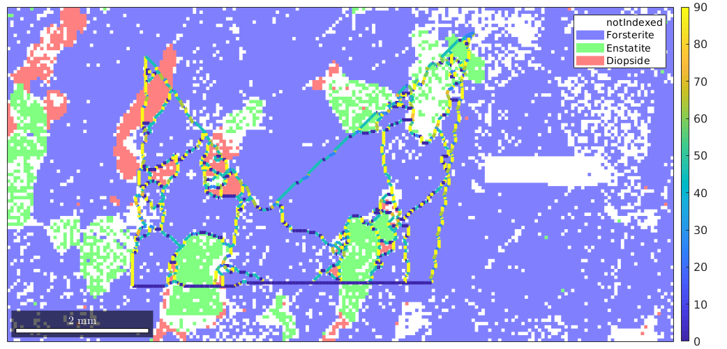
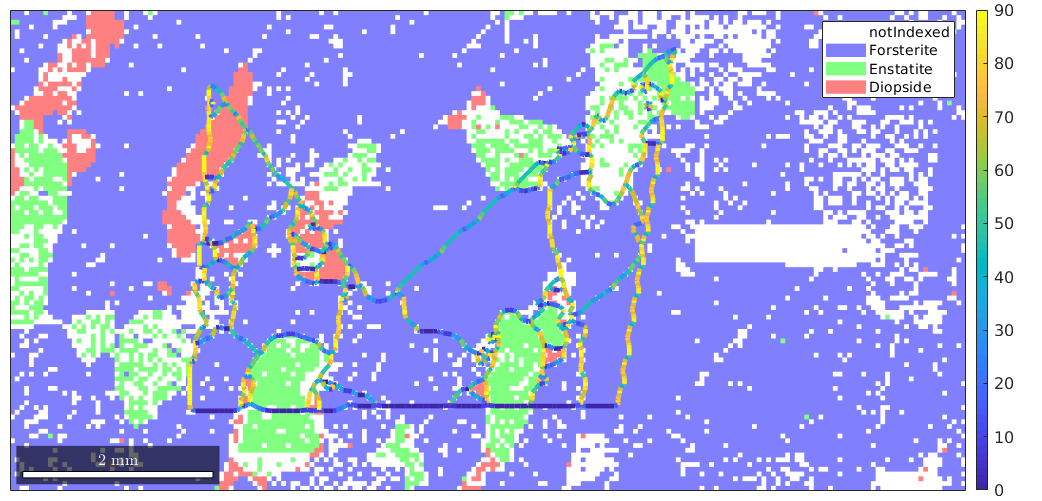
We see that the angle between the grain boundary direction and the x-axis takes only values 0, 45 and 90 degrees. After applying smoothing we obtain a much better result
% smooth the grain boundaries
grains = smooth(grains)

% plot the raw data
plot(ebsd)

% start overide mode
hold on

% plot the boundary of all grains
plot(grains.boundary,angle(grains.boundary.direction,xvector)./degree,'linewidth',3.5)
mtexColorbar

% stop overide mode
hold off
grains = grain2d

 Phase  Grains  Pixels     Mineral  Symmetry  Crystal reference frame
     1      28    2756  Forsterite       mmm
     2       9     452   Enstatite       mmm
     3      22     231    Diopside     12/m1       X||a*, Y||b*, Z||c

 boundary segments: 1252
 triple points: 61

 Properties: GOS, meanRotation
Grain reconstruction by the multiscale clustering method
When analyzing grains with gradual and subtle boundaries the threshold based method may not lead to the desired result.
Let us consider the following example
mtexdata single

ipfKey = axisAngleColorKey(ebsd);
ipfKey.oriRef = mean(ebsd.orientations);

plot(ebsd,ipfKey.orientation2color(ebsd.orientations))
loading data ... saving data to /home/hielscher/mtex/master/data/single.mat
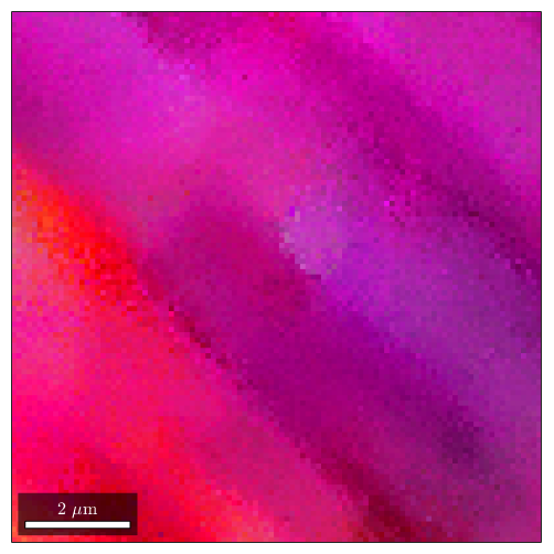
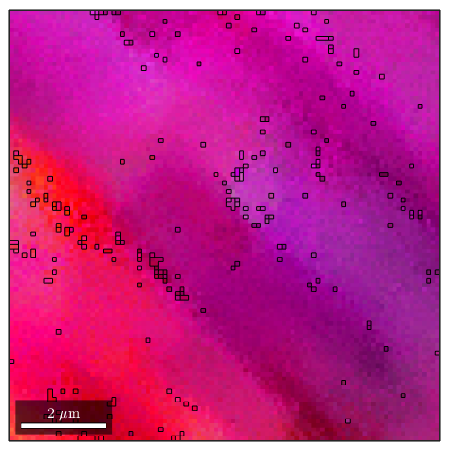
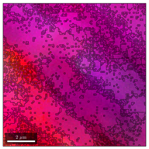
We obeserve that the are no rapid changes in the orientation which would allow for applying the threshold based algorithm. Setting the threshold angle to a very small value would include many irrelevant or false regions.
grains_high = calcGrains(ebsd,'angle',1*degree);
grains_low  = calcGrains(ebsd,'angle',0.5*degree);

figure
plot(ebsd,ipfKey.orientation2color(ebsd.orientations))
hold on
plot(grains_high.boundary)
hold off

figure
plot(ebsd,ipfKey.orientation2color(ebsd.orientations))
hold on
plot(grains_low.boundary)
hold off
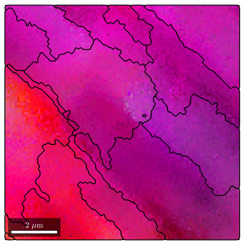
As an alternative MTEX includes the fast multiscale clustering method (FMC method) which constructs clusters in a hierarchical manner from single pixels using fuzzy logic to account for local, as well as global information.
Analogous with the threshold angle, a single parameter, C_Maha controls the sensitivity of the segmentation. A C_Maha value of 3.5 properly identifies the subgrain features. A C_Maha value of 3 captures more general features, while a value of 4 identifies finer features but is slightly oversegmented.
grains_FMC = calcGrains(ebsd('indexed'),'FMC',3.8)
grains = calcGrains(ebsd('indexed'))

% smooth grains to remove staircase effect
grains_FMC = smooth(grains_FMC);
grains_FMC = grain2d

 Phase  Grains  Pixels  Mineral  Symmetry  Crystal reference frame
     1      17   10201       Al      m-3m

 boundary segments: 1552
 triple points: 14

 Id   Phase   Pixels          GOS   phi1   Phi   phi2
  1       1        7   0.00851854    318   128    159
  2       1     1120    0.0238482    239    75    320
  3       1      517    0.0100044    238    76    320
  4       1     1783    0.0220796     56   103     40
  5       1       11   0.00748579     57   104    221
  6       1        2   0.00276888    237    79    322
  7       1        7   0.00810474    343    43    249
  8       1      989    0.0126317    236    79    322
  9       1     1060    0.0197436    239    75    320
 10       1       76   0.00792457    238    75    320
 11       1     1556    0.0218341    238    77    320
 12       1      349    0.0114275    237    77    320
 13       1      401    0.0103653    342    41    252
 14       1      402     0.012066    238    77    320
 15       1      184    0.0128148    237    77    319
 16       1      957    0.0175949    316   129     74
 17       1      780    0.0122539    238    78    321


grains = grain2d

 Phase  Grains  Pixels  Mineral  Symmetry  Crystal reference frame
     1       1   10201       Al      m-3m

 boundary segments: 404
 triple points: 0

 Id   Phase   Pixels         GOS   phi1   Phi   phi2
  1       1    10201   0.0343764    237    77    320
We observe how this method nicely splits the measurements into clusters of similar orientation
%plot(ebsd,oM.orientation2color(ebsd.orientations))
plot(ebsd,ipfKey.orientation2color(ebsd.orientations))

% start overide mode
hold on
plot(grains_FMC.boundary,'linewidth',1.5)

% stop overide mode
hold off
TESTING OMLY
Below this is some testing code as the FMC method does not work so satisfactory in the present example
F = halfQuadraticFilter
F.alpha = 0.01;
F.eps = 1e-5;
F.tol = 1e-10;

ebsdS = smooth(ebsd('indexed'),F)
F =
halfQuadraticFilter with properties:
alpha: [0.1000 0.1000]
weight: @(t,eps,th)(t<=th)./(t.^2+eps^2).^(1/2)
eps: 0.0100
tol: 1.0000e-05
threshold: 0.0873
ebsdS = EBSD
Phase Orientations Mineral Color Symmetry Crystal reference frame
1 10201 (100%) Al light blue m-3m
Properties: x, y
Scan unit : um
[grains_FMC,ebsdS.grainId] = calcGrains(ebsdS('indexed'),'FMC',2)

% smooth grains to remove staircase effect
grains_FMC = smooth(grains_FMC)
grains_FMC = grain2d

 Phase  Grains  Pixels  Mineral  Symmetry  Crystal reference frame
     1      63   10201       Al      m-3m

 boundary segments: 2344
 triple points: 58

 Properties: GOS, meanRotation


ebsdS = EBSD

 Phase  Orientations  Mineral       Color  Symmetry  Crystal reference frame
     1  10201 (100%)       Al  light blue      m-3m

 Properties: x, y, grainId
 Scan unit : um


grains_FMC = grain2d

 Phase  Grains  Pixels  Mineral  Symmetry  Crystal reference frame
     1      63   10201       Al      m-3m

 boundary segments: 2344
 triple points: 58

 Properties: GOS, meanRotation
plot(ebsdS('indexed'),ipfKey.orientation2color(ebsdS('indexed').orientations))


hold on
plot(grains_FMC.boundary)
hold off
[grains,ebsdS.grainId] = calcGrains(ebsdS('indexed'),'angle',0.5*degree);
ebsdS(grains(grains.grainSize<=3)) = [];

[grains,ebsdS.grainId] = calcGrains(ebsdS('indexed'),'angle',0.25*degree);
grains
grains = grain2d

 Phase  Grains  Pixels  Mineral  Symmetry  Crystal reference frame
     1     241   10012       Al      m-3m

 boundary segments: 2024
 triple points: 265

 Properties: GOS, meanRotation
plot(ebsdS('indexed'),ipfKey.orientation2color(ebsdS('indexed').orientations))


hold on
plot(grains.boundary)
hold off
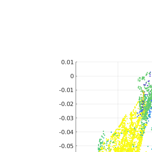
ori = ebsdS('indexed').orientations;
meanOri = mean(ori)
grainId = ebsdS('indexed').grainId;

v = axis(ori,meanOri) .* angle(ori,meanOri);

vv = v(grainId==2);
scatter3(v.x,v.y,v.z,10*ones(size(grainId)),grainId,'filled')
fcw
hold on
scatter3(vv.x,vv.y,vv.z,10,'MarkerFaceColor','red')
meanOri = orientation
  size: 1 x 1
  crystal symmetry : Al (m-3m)
  specimen symmetry: 1

  Bunge Euler angles in degree
     phi1     Phi    phi2    Inv.
  345.437 37.1383 337.793       0
| DocHelp 0.1 beta |