Misorientation Analysis
How to analyze misorientations.
Definition
In MTEX the misorientation between two orientations o1, o2 is defined as
In the case of EBSD data, intragranular misorientations, misorientations between neighbouring grains, and misorientations between random measurements are of interest.
The sample data set
Let us first import some EBSD data by a script file
mtexdata forsterite
plotx2east
and reconstruct grains by
% perform grain segmentation
[grains,ebsd.grainId,ebsd.mis2mean] = calcGrains(ebsd('indexed'),'threshold',5*degree);

% remove small grains
ebsd(grains(grains.grainSize<5)) = [];

% repeat grain reconstruction
[grains,ebsd.grainId,ebsd.mis2mean] = calcGrains(ebsd('indexed'),'threshold',5*degree);

% smooth the grain boundaries a bit
grains = smooth(grains,5);
Intragranular misorientations
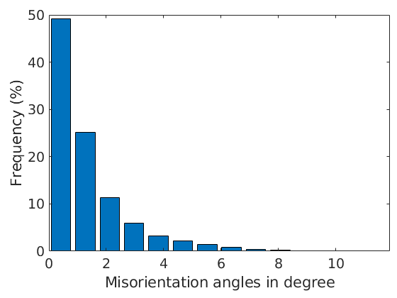
The intragranular misorientation is automatically computed while reconstructing the grain structure. It is stored as the property mis2mean within the ebsd variable and can be accessed by
% get the misorientations to mean
mori = ebsd('Fo').mis2mean

% plot a histogram of the misorientation angles
plotAngleDistribution(mori)
xlabel('Misorientation angles in degree')
mori = misorientation
  size: 151452 x 1
  crystal symmetry : Forsterite (mmm)
  crystal symmetry : Forsterite (mmm)
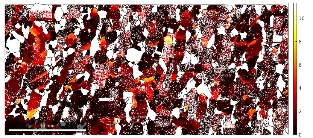
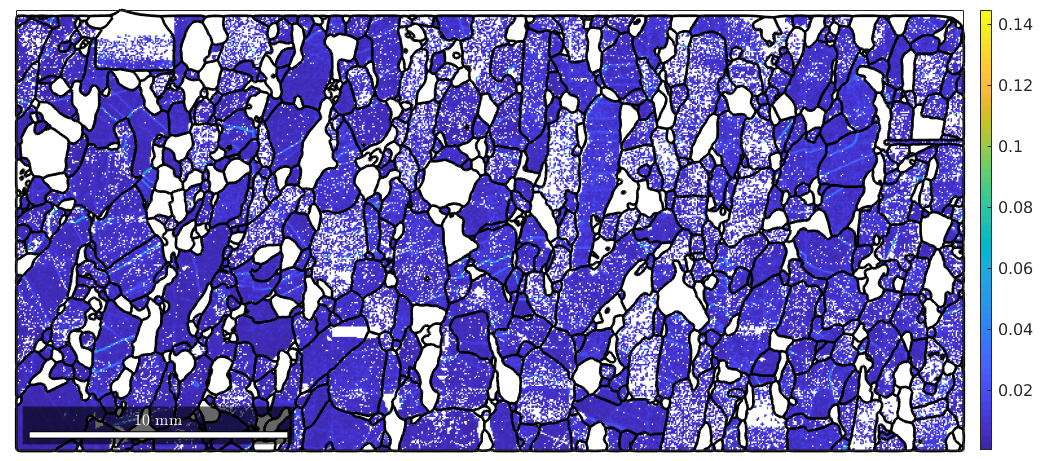
The visualization of the misorientation angle can be done by
close all
plot(ebsd('Forsterite'),ebsd('Forsterite').mis2mean.angle./degree)
mtexColorMap hot
mtexColorbar
hold on
plot(grains.boundary,'edgecolor','k','linewidth',.5)
hold off
In order to visualize the misorientation axis we have two choices. We can consider the misorientation axis either with respect to the crystal reference frame or with the specimen reference frame. The misorientation axes with respect to the crystal reference frame can be computed via
mori.axis
ans = Miller
 size: 151452 x 1
 mineral: Forsterite (222)
The axes are unique up to crystal symmetry. Accordingly, the corresponding color key needs to colorize only the fundamental sector. This is done by
% define the color key
oM = axisAngleColorKey(mori);

plot(oM)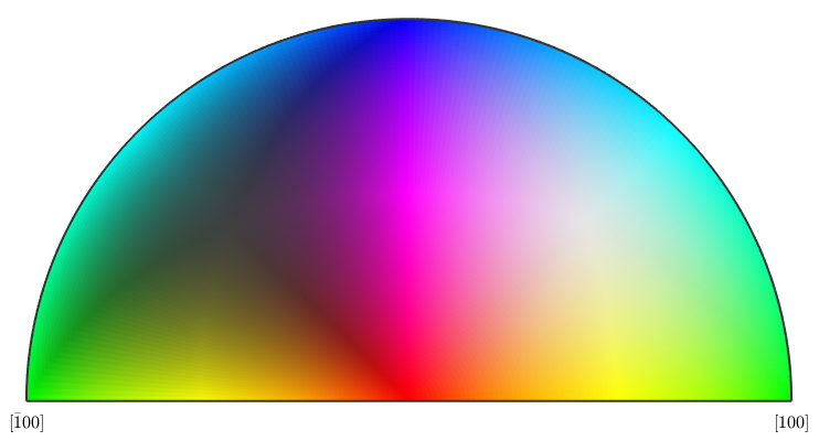
We see that according to the above color key orientation gradients with respect to the (001) axis will be displayed in red, spins around the (010) will be displayed in green and spins around the (100) axis will be displayed in blue. Pixels with no misorientation will be displayed in gray and as the misorientation angle increases the color gets more saturated.
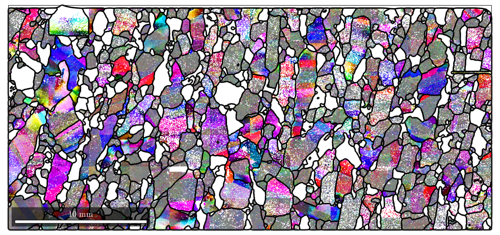
plot(ebsd('Forsterite'),oM.orientation2color(mori))

hold on
plot(grains.boundary,'edgecolor','k','linewidth',2)
hold off
The misorientation axis with respect to the specimen coordinate system can unfortunaltely not be computed from the misorientation alone. Therefore, we require the pair consisting of grain mean orientation and the orientation of the pixel.
Lets computed first for every pixel the corresponding reference orientation, i.e. the mean orientation of the grain the pixel belongs to.
oriRef = grains(ebsd('Forsterite').grainId).meanOrientationoriRef = orientation size: 151452 x 1 crystal symmetry : Forsterite (mmm) specimen symmetry: 1
Now the misorientation axis with respect to the specimen reference system is computed via
v = axis(ebsd('Forsterite').orientations,oriRef)v = vector3d size: 151452 x 1
With respect to the specimen reference frame the misorientation axes are unique and not symmetry has to be considered. Accordingly, our color key will contain the entire sphere.
oM = axisAngleColorKey(ebsd('Forsterite'));
plot(oM)

plot(discreteSample(v,1000),'add2all','MarkerSize',2,'MarkerEdgeColor','black')
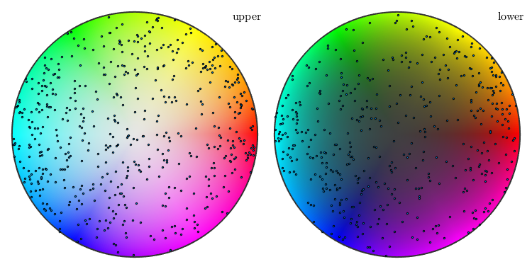
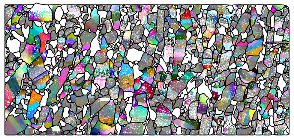
With respect to the above color key rotations around the 001 specimen direction will become visible as a black to white gradient while rotations around the 100 directions will show up as a red to magenta gradient.
oM.oriRef = oriRef;

color = oM.orientation2color(ebsd('Forsterite').orientations);
plot(ebsd('Forsterite'),color,'micronbar','off')
hold on
plot(grains.boundary,'edgecolor','k','linewidth',2)
hold off
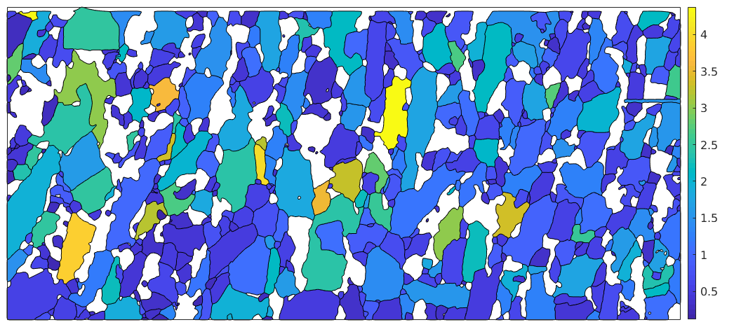
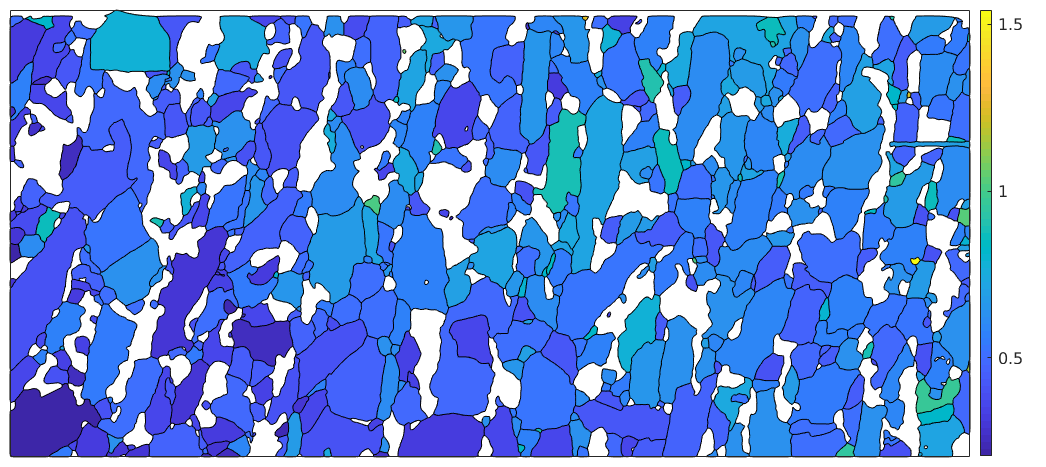
Grain orientation spread (GOS)
plot(grains('fo'),grains('fo').GOS./degree,'micronbar','off')
mtexColorbar
Kernel average misorientation (KAM)
KAM = ebsd('fo').KAM;
plot(ebsd('fo'),KAM);
mtexColorbar
hold on
plot(grains.boundary,'linewidth',2)
hold off
Grain average misorientation (GAM)
The grain average misorientation (GAM) is defined as the mean KAM within each grain. The following line can be taken as a blueprint how to average arbitrary properties within grains. The last argument @nanmean in this command indicates that the average should be taken as the mean ignoring NaNs. In order to a assign the maximum value to each grain replace this with @max.
GAM = accumarray(ebsd('fo').grainId, KAM, size(grains), @nanmean) ./degree;% plot the GAM plot(grains('fo'),GAM(grains('fo').id),'micronbar','off') mtexColorbar
Boundary misorientations
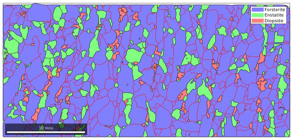
The misorientation between adjacent grains can be computed by the command grainBoundary.misorientation.html
plot(grains)

hold on

bnd_FoFo = grains.boundary('Fo','Fo')

plot(bnd_FoFo,'linecolor','r')

hold off

bnd_FoFo.misorientation
bnd_FoFo = grainBoundary

 Segments   mineral 1   mineral 2
    15676  Forsterite  Forsterite

ans = misorientation
  size: 15676 x 1
  crystal symmetry : Forsterite (mmm)
  crystal symmetry : Forsterite (mmm)
  antipodal:         true
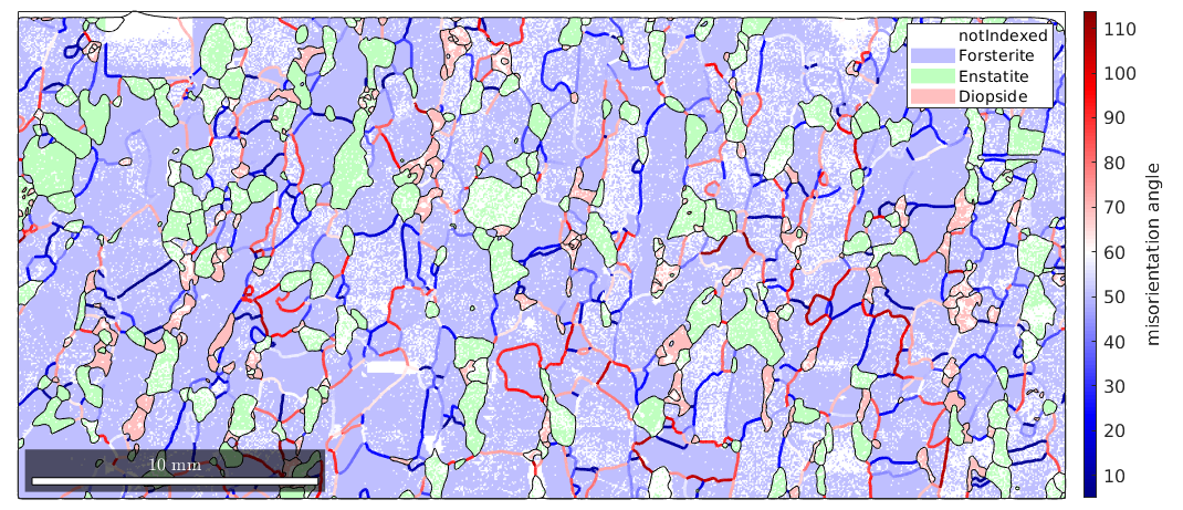
plot(ebsd,'facealpha',0.5)

hold on
plot(grains.boundary)
plot(bnd_FoFo,bnd_FoFo.misorientation.angle./degree,'linewidth',2)
mtexColorMap blue2red
mtexColorbar('title','misorientation angle')
hold off
In order to visualize the misorientation between any two adjacent grains, there are two possibilities in MTEX.
- plot the angle distribution for all phase combinations
- plot the axis distribution for all phase combinations
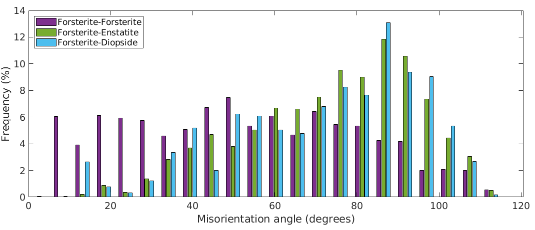
The angle distribution
The following commands plot the angle distributions of all phase transitions from Forsterite to any other phase.
plotAngleDistribution(grains.boundary('Fo','Fo').misorientation,...
  'DisplayName','Forsterite-Forsterite')
hold on
plotAngleDistribution(grains.boundary('Fo','En').misorientation,...
  'DisplayName','Forsterite-Enstatite')
plotAngleDistribution(grains.boundary('Fo','Di').misorientation,...
  'DisplayName','Forsterite-Diopside')
hold off
legend('show','Location','northwest')
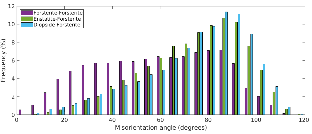
The above angle distributions can be compared with the uncorrelated misorientation angle distributions. This is done by
% compute uncorrelated misorientations
mori = calcMisorientation(ebsd('Fo'),ebsd('Fo'));

% plot the angle distribution
plotAngleDistribution(mori,'DisplayName','Forsterite-Forsterite')

hold on

mori = calcMisorientation(ebsd('Fo'),ebsd('En'));
plotAngleDistribution(mori,'DisplayName','Forsterite-Enstatite')

mori = calcMisorientation(ebsd('Fo'),ebsd('Di'));
plotAngleDistribution(mori,'DisplayName','Forsterite-Diopside')

hold off
legend('show','Location','northwest')
Another possibility is to compute an uncorrelated angle distribution from EBSD data by taking only into account those pairs of measurements that are sufficiently far from each other (uncorrelated points). The uncorrelated angle distribution is plotted by
% compute the Forsterite ODF
odf_Fo = calcODF(ebsd('Fo').orientations,'Fourier')

% compute the uncorrelated Forsterite to Forsterite MDF
mdf_Fo_Fo = calcMDF(odf_Fo,odf_Fo)

% plot the uncorrelated angle distribution
hold on
plotAngleDistribution(mdf_Fo_Fo,'DisplayName','Forsterite-Forsterite')
hold off

legend('-dynamicLegend','Location','northwest') % update legend
odf_Fo = ODF
  crystal symmetry : Forsterite (mmm)
  specimen symmetry: 1

  Harmonic portion:
    degree: 25
    weight: 1


mdf_Fo_Fo = MDF
  crystal symmetry : Forsterite (mmm)
  crystal symmetry : Forsterite (mmm)
  antipodal:         true

  Harmonic portion:
    degree: 20
    weight: 1
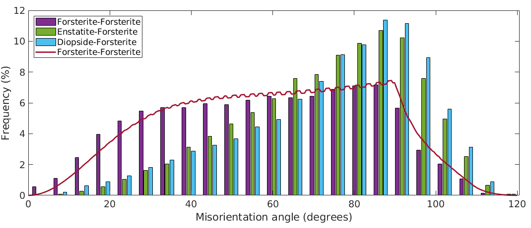
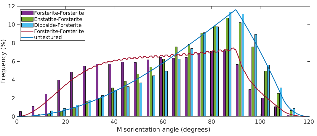
What we have plotted above is the uncorrelated misorientation angle distribution for the Forsterite ODF. We can compare it to the uncorrelated misorientation angle distribution of the uniform ODF by
hold on
plotAngleDistribution(odf_Fo.CS,odf_Fo.CS,'DisplayName','untextured')
hold off

legend('-dynamicLegend','Location','northwest') % update legend
The axis distribution
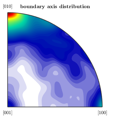
Let's start with the boundary misorientation axis distribution
close all
plotAxisDistribution(bnd_FoFo.misorientation,'smooth')
mtexTitle('boundary axis distribution')
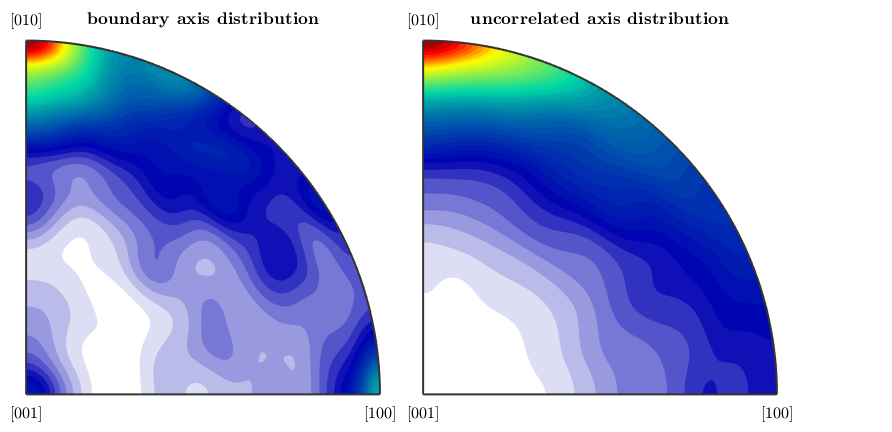
Next we plot with the uncorrelated axis distribution, which depends only on the underlying ODFs.
nextAxis
mori = calcMisorientation(ebsd('Fo'));
plotAxisDistribution(mori,'smooth')
mtexTitle('uncorrelated axis distribution')
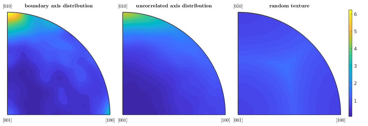
and finally the axis misorientation distribution of a random texture
nextAxis
plotAxisDistribution(ebsd('Fo').CS,ebsd('Fo').CS,'antipodal')
mtexTitle('random texture')
mtexColorMap parula
setColorRange('equal')
mtexColorbar('multiples of random distribution')
| DocHelp 0.1 beta |