Dislocation Density Estimation
This example sheet describes how to estimate dislocation densities in MTEX following the reference paper
Pantleon, Resolving the geometrically necessary dislocation content by conventional electron backscattering diffraction, Scripta Materialia, 2008
Data import and grain reconstruction
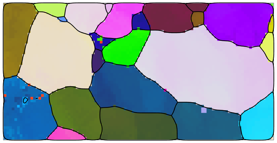
Lets start by importing orientation data from 2 percent uniaxial deformed steel DC06 and visualize those data in an ipf map.
% set up the plotting convention
plotx2north

% import the EBSD data
ebsd = EBSD.load([mtexDataPath filesep 'EBSD' filesep 'DC06_2uniax.ang']);
%ebsd = EBSD.load('DC06_2biax.ang');

% define the color key
ipfKey = ipfHSVKey(ebsd);
ipfKey.inversePoleFigureDirection = yvector;

% and plot the orientation data
plot(ebsd,ipfKey.orientation2color(ebsd.orientations),'micronBar','off','figSize','medium')

In the next step we reconstruct grains, remove all grains with less then 5 pixels and smooth the grain boundaries.
% reconstruct grains
[grains,ebsd.grainId] = calcGrains(ebsd,'angle',5*degree);

% remove small grains
ebsd(grains(grains.grainSize<=5)) = [];

% redo grain reconstruction
[grains,ebsd.grainId] = calcGrains(ebsd,'angle',2.5*degree);

% smooth grain boundaries
grains = smooth(grains,5);

hold on
plot(grains.boundary,'linewidth',2)
hold off
Data cleaning
The computation of geometrically neccesary dislocations from EBSD maps depends on local orientation changes in the map. In order to make those visible we switch to a different color key that colorises the misorientation of an pixel with respect to the grain meanorientation.
% a key the colorizes according to misorientation angle and axis
ipfKey = axisAngleColorKey(ebsd);

% set the grain mean orientations as reference orinetations
ipfKey.oriRef = grains(ebsd('indexed').grainId).meanOrientation;

% plot the data
plot(ebsd,ipfKey.orientation2color(ebsd('indexed').orientations),'micronBar','off','figSize','medium')

hold on
plot(grains.boundary,'linewidth',2)
hold off
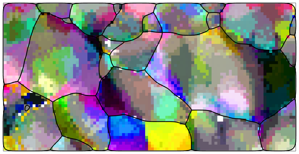
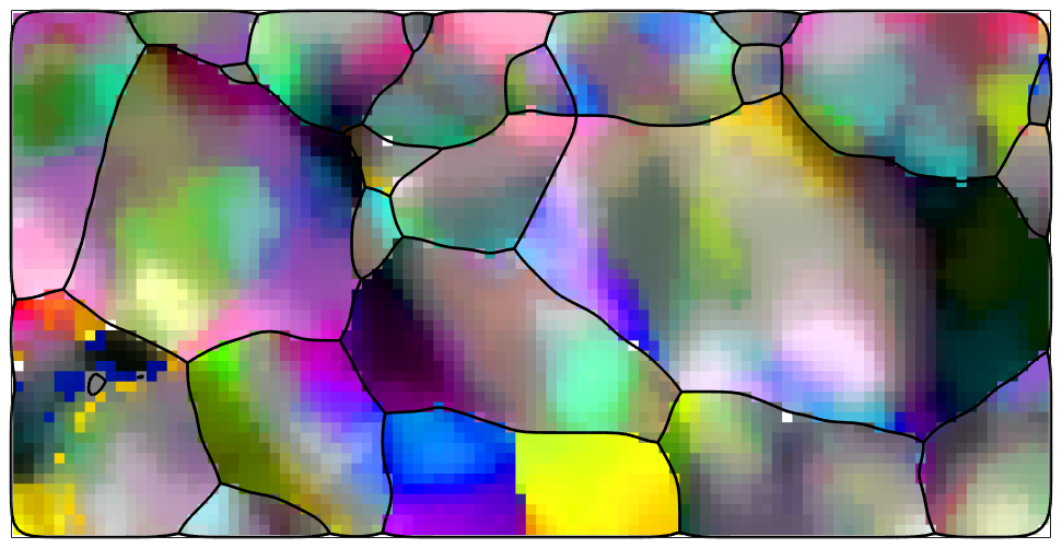
We observe that the data are quite noisy. As noisy orientation data lead to overestimate the GND density we apply sime denoising techniques to the data.
% denoise orientation data
F = halfQuadraticFilter;
F.threshold = 1.5*degree;
F.eps = 1e-2;
F.alpha = 0.01;
ebsd = smooth(ebsd('indexed'),F,'fill',grains);

% plot the denoised data
ipfKey.oriRef = grains(ebsd('indexed').grainId).meanOrientation;
plot(ebsd('indexed'),ipfKey.orientation2color(ebsd('indexed').orientations),'micronBar','off','figSize','medium')

hold on
plot(grains.boundary,'linewidth',2)
hold off
denoising EBSD data: 100%
The incomplete curvature tensor
Starting point of any GND computation is the curvature tensor, which is a rank two tensor that is defined for every pixel in the EBSD map by the directional derivatives in x, y and z direction.
% consider only the Fe(alpha) phase
ebsd = ebsd('indexed').gridify;

% compute the curvature tensor
kappa = ebsd.curvature

% one can index the curvature tensors in the same way as the EBSD data.
% E.g. the curvature in pixel (2,3) is
kappa(2,3)
kappa = curvatureTensor
  size: 101 x 51
  unit: 1/um
  rank: 2 (3 x 3)

ans = curvatureTensor
  unit: 1/um
  rank: 2 (3 x 3)

 *10^-4
   1.767  15.127     NaN
  -5.178   1.493     NaN
 -12.003  16.171     NaN
The components of the curvature tensor
As expected the curvature tensor is NaN in the third column as this column corresponds to the directional derivative in z-direction which is usually unknown for 2d EBSD maps.
We can access the different components of the curvature tensor with
kappa12 = kappa{1,2};

size(kappa12)
ans = 101 51
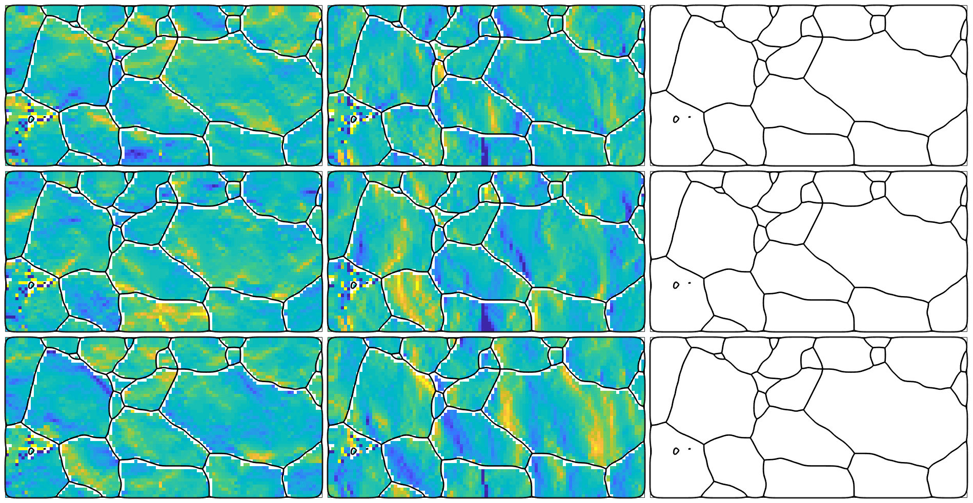
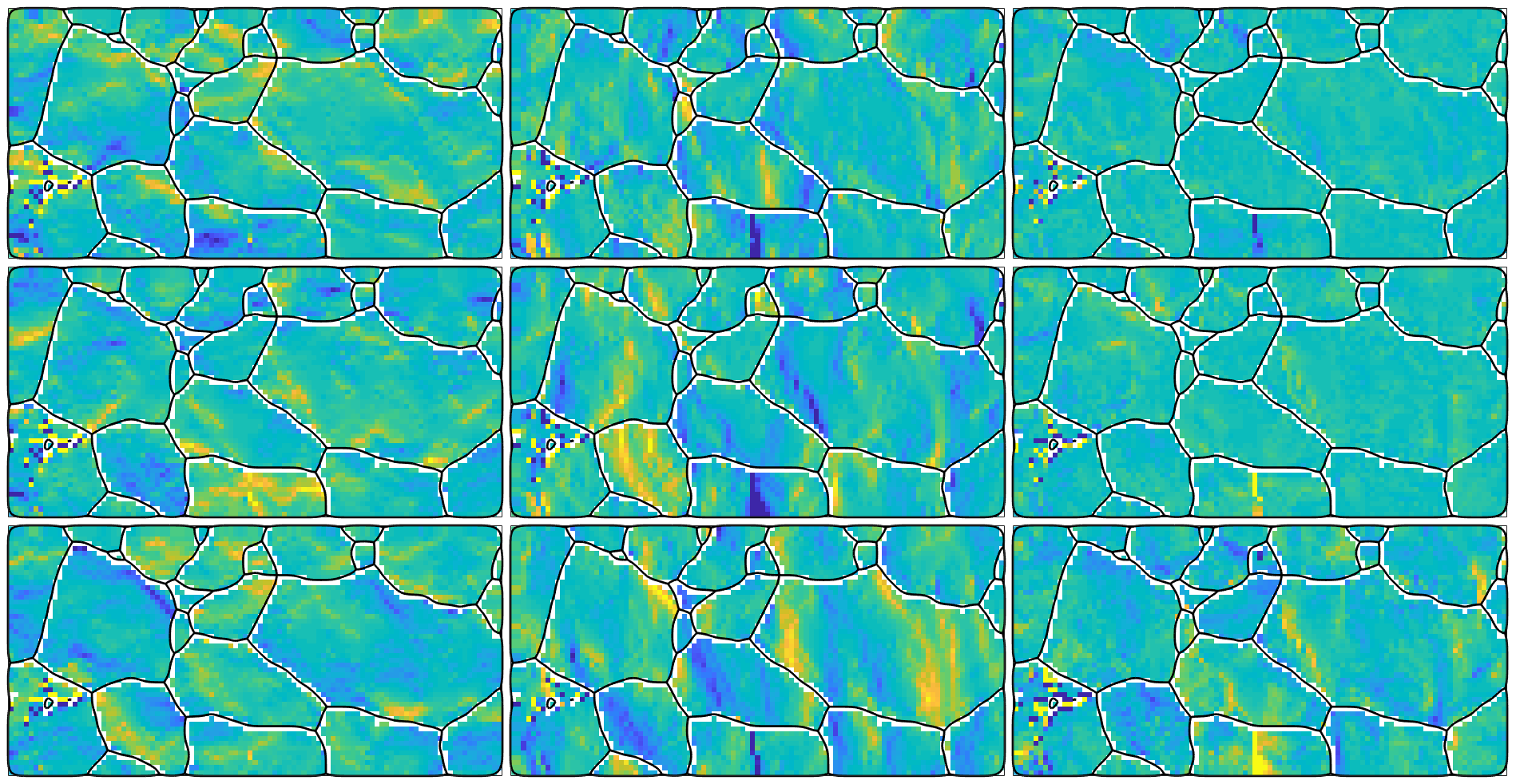
which results in a variable of the same size as our EBSD map. This allows us to visualize the different components of the curvature tensor
newMtexFigure('nrows',3,'ncols',3);

% cycle through all components of the tensor
for i = 1:3
  for j = 1:3

    nextAxis(i,j)
    plot(ebsd,kappa{i,j},'micronBar','off')
    hold on; plot(grains.boundary,'linewidth',2); hold off

  end
end

% unify the color rage  - you may also use setColoRange equal
setColorRange([-0.005,0.005])
drawNow(gcm,'figSize','large')
The incomplete dislocation density tensor
According to Kroener the curvature tensor is directly related to the dislocation density tensor.
alpha = kappa.dislocationDensity
alpha = dislocationDensityTensor
  size: 101 x 51
  unit: 1/um
  rank: 2 (3 x 3)
which has the same unit as the curvature tensor and is incomplete as well as we can see when looking at a particular one.
alpha(2,3)
ans = dislocationDensityTensor
  unit: 1/um
  rank: 2 (3 x 3)

 *10^-4
     NaN  -5.178 -12.003
  15.127     NaN  16.171
     NaN     NaN   -3.26
Crystallographic Dislocations
The central idea of Pantleon is that the dislocation density tensor is build up by single dislocations with different densities such that the total energy is minimum. Depending on the attomic lattice different dislocattion systems have to be considered. In present case of a body centered cubic (bcc) material 48 edge dislocations and 4 screw dislocations have to be considered. Those principle dislocations are defined in MTEX either by their Burgers and line vectors or by
dS = dislocationSystem.bcc(ebsd.CS)
dS = dislocationSystem
 mineral: Iron (Alpha) (432)
 edge dislocations : 48 x 1
 Burgers vector  line vector  energy
      [1 -1  1]   (-2 -1  1)       2
      [1  1 -1]    (2 -1  1)       2
      [1  1 -1]    (1 -2 -1)       2
     [-1  1  1]    (1  2 -1)       2
      [1 -1  1]   (-1  1  2)       2
     [-1  1  1]   (-1  1 -2)       2
      [1 -1  1]    (1  2  1)       2
      [1  1  1]   (-1  2 -1)       2
      [1  1 -1]    (1  1  2)       2
      [1  1  1]   (-1 -1  2)       2
     [-1  1  1]    (2  1  1)       2
      [1  1  1]    (2 -1 -1)       2
     [-1  1  1]    (0  1 -1)       2
      [1 -1  1]   (-1  0  1)       2
      [1  1 -1]    (1 -1  0)       2
     [-1  1  1]   (-1  0 -1)       2
      [1 -1  1]   (-1 -1  0)       2
      [1  1 -1]    (0 -1 -1)       2
      [1  1 -1]    (1  0  1)       2
     [-1  1  1]    (1  1  0)       2
      [1 -1  1]    (0  1  1)       2
     [-1 -1 -1]    (0 -1  1)       2
     [-1 -1 -1]    (1  0 -1)       2
     [-1 -1 -1]   (-1  1  0)       2
     [-1  1  1]   (-1  4 -5)       2
      [1 -1  1]   (-5 -1  4)       2
      [1  1 -1]    (4 -5 -1)       2
     [-1  1  1]   (-4  1 -5)       2
      [1 -1  1]   (-5 -4  1)       2
      [1  1 -1]    (1 -5 -4)       2
      [1  1 -1]    (4  1  5)       2
     [-1  1  1]    (5  4  1)       2
      [1 -1  1]    (1  5  4)       2
     [-1 -1 -1]   (-1 -4  5)       2
     [-1 -1 -1]    (5 -1 -4)       2
     [-1 -1 -1]   (-4  5 -1)       2
      [1 -1  1]    (1 -4 -5)       2
      [1  1 -1]   (-5  1 -4)       2
     [-1  1  1]   (-4 -5  1)       2
      [1 -1  1]    (4 -1 -5)       2
      [1  1 -1]   (-5  4 -1)       2
     [-1  1  1]   (-1 -5  4)       2
     [-1 -1 -1]   (-4 -1  5)       2
     [-1 -1 -1]    (5 -4 -1)       2
     [-1 -1 -1]   (-1  5 -4)       2
      [1  1 -1]    (1  4  5)       2
     [-1  1  1]    (5  1  4)       2
      [1 -1  1]    (4  5  1)       2

 screw dislocations: 4 x 1
 Burgers vector  energy
     (-1 -1 -1)       1
      (1 -1  1)       1
     (-1  1  1)       1
      (1  1 -1)       1
Here the norm of the Burgers vectors is important
% size of the unit cell
a = norm(ebsd.CS.aAxis);

% in bcc and fcc the norm of the burgers vector is sqrt(3)/2 * a
[norm(dS(1).b), norm(dS(end).b), sqrt(3)/2 * a]
ans =
    2.4855    2.4855    2.4855
The Energy of Dislocations
The energy of each dislocation system can be stored in the property u. By default this value it set to 1 but should be changed accoring to the specific model and the specific material.
According to Hull & Bacon the energy U of edge and screw dislocations is given by the formulae
$$ U_{\text{screw}} = \frac{Gb^2}{4\pi} \ln \frac{R}{r_0} $$
Error updating Text.

 String scalar or character vector must have valid interpreter syntax:
$$ U_{\text{screw}} = \frac{Gb^2}{4\pi} \ln \frac{R}{r_0} $$
$$ U_{\text{edge}} = (1-\nu) U_{\text{screw}} $$
Error updating Text.

 String scalar or character vector must have valid interpreter syntax:
$$ U_{\text{edge}} = (1-\nu) U_{\text{screw}} $$
where
- G is
- b is the length of the Burgers vector
- nu is the Poisson ratio
- R
- r
In this example we assume
%
%R =
%r_0 =
%U = norm(dS.b).^2

nu = 0.3;


% energy of the edge dislocations
dS(dS.isEdge).u = 1;

% energy of the screw dislocations
dS(dS.isScrew).u = 1 - 0.3;

% Question to verybody: what is the best way to set the enegry? I found
% different formulae
%
% E = 1 - poisson ratio
% E = c * G * |b|^2,  - G - Schubmodul / Shear Modulus Energy per (unit length)^2
A single dislocation causes a deformation that can be represented by the rank one tensor
dS(1).tensor
ans = dislocationDensityTensor
  unit   : au
  rank   : 2 (3 x 3)
  mineral: Iron (Alpha) (432)

 -1.1717 -0.5858  0.5858
  1.1717  0.5858 -0.5858
 -1.1717 -0.5858  0.5858
Note that the unit of this tensors is the same as the unit used for describing the length of the unit cell, which is in most cases Angstrom (au). Furthremore, we observe that the tensor is given with respect to the crystal reference frame while the dislocation densitiy tensors are given with respect to the specimen reference frame. Hence, to make them compatible we have to rotate the dislocation tensors into the specimen reference frame as well. This is done by
dSRot = ebsd.orientations * dS
dSRot = dislocationSystem
 edge dislocations : 5144 x 48
 screw dislocations: 5144 x 4
Fitting Dislocations to the incomplete dislocation density tensor
Now we are ready for fitting the dislocation tensors to the dislocation densitiy tensor in each pixel of the map. This is done by the command fitDislocationSystems.
[rho,factor] = fitDislocationSystems(kappa,dSRot);
Optimal solution found.

 fitting: 100%
As result we obtain a matrix of densities rho such that the product with the dislocation systems yields the incomplete dislocation density tensors derived from the curvature, i.e.,
% the restored dislocation density tensors
alpha = sum(dSRot.tensor .* rho,2);

% we have to set the unit manualy since it is not stored in rho
alpha.opt.unit = '1/um';

% the restored dislocation density tensor for pixel 2
alpha(2)

% the dislocation density dervied from the curvature in pixel 2
kappa(2).dislocationDensity
ans = dislocationDensityTensor
  unit: 1/um
  rank: 2 (3 x 3)

 *10^-5
 -22.73   1.96 -29.17
  48.71   6.38  44.63
  -5.15   1.79   5.26

ans = dislocationDensityTensor
  unit: 1/um
  rank: 2 (3 x 3)

 *10^-5
    NaN   1.96 -29.17
  48.71    NaN  44.63
    NaN    NaN   5.26
we may also restore the complete curvature tensor with
kappa = alpha.curvature
kappa = curvatureTensor
  size: 5151 x 1
  unit: 1/um
  rank: 2 (3 x 3)
and plot it as we did before
newMtexFigure('nrows',3,'ncols',3);

% cycle through all components of the tensor
for i = 1:3
  for j = 1:3

    nextAxis(i,j)
    plot(ebsd,kappa{i,j},'micronBar','off')
    hold on; plot(grains.boundary,'linewidth',2); hold off

  end
end

setColorRange([-0.005,0.005])
drawNow(gcm,'figSize','large');
The total dislocation energy
The unit of the densities h in our example is 1/um * 1/au where 1/um comes from the unit of the curvature tensor an 1/au from the unit of the Burgers vector. In order to transform h to SI units, i.e., 1/m^2 we have to multiply it with 10^16. This is exactly the values returned as the second output factor by the function fitDislocationSystems.
factor
factor =
   1.0000e+16
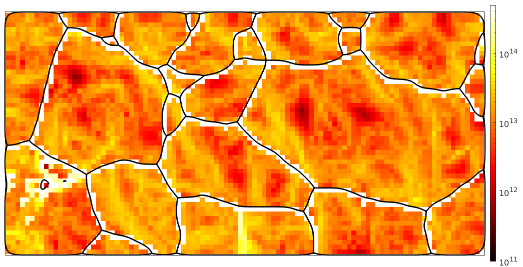
Multiplying the densities rho with this factor and the individual energies of the the dislocation systems we end up with the total dislocation energy. Lets plot this at a logarithmic scale
close all
plot(ebsd,factor*sum(abs(rho .* dSRot.u),2),'micronbar','off')
mtexColorMap('hot')
mtexColorbar

set(gca,'ColorScale','log'); % this works only starting with Matlab 2018a
set(gca,'CLim',[1e11 5e14]);

hold on
plot(grains.boundary,'linewidth',2)
hold off
plotx2east
| DocHelp 0.1 beta |