Plotting spatially indexed EBSD data

How to visualize EBSD data

This section gives you an overview of the functionality MTEX offers to visualize spatial orientation data.

Phase Plots

Visualizing arbitrary properties

Visualizing orientations

Customizing the color

Coloring certain fibres

Coloring certain orientations

Combining different plots

Phase Plots

Let us first import some EBSD data with a script file

close all; plotx2east
mtexdata forsterite
csFo = ebsd('Forsterite').CS

 
csFo = crystalSymmetry  
 
  mineral : Forsterite
  color   : light blue
  symmetry: mmm       
  a, b, c : 4.8, 10, 6

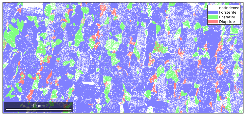
By default, MTEX plots a phase map for EBSD data.

plot(ebsd)

You can access the color of each phase by

ebsd('Diopside').color

ans =
    1.0000    0.5000    0.5000

These values are RGB values, e.g. to make the color for diopside even more red we can do

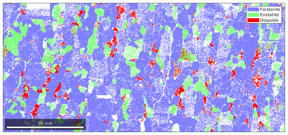
ebsd('Diopside').color = [1 0 0];

plot(ebsd('indexed'))

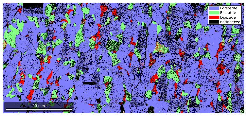
By default, not indexed phases are plotted as white. To directly specify a color for some EBSD data use the option FaceColor.

hold on
plot(ebsd('notIndexed'),'FaceColor','black')
hold off

Visualizing arbitrary properties

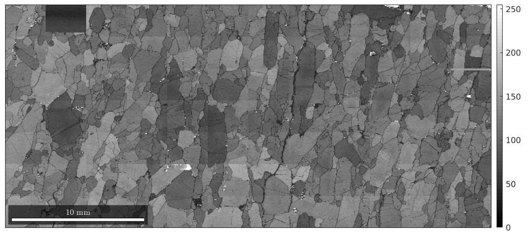
Apart from the phase information, we can use any other property to colorize the EBSD data. As an example, we may plot the band contrast

plot(ebsd,ebsd.bc)

colormap gray % this makes the image grayscale

mtexColorbar

Visualizing orientations

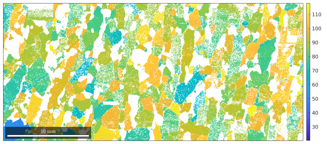
Actually, we can pass any list of numbers or colors as a second input argument to be visualized together with the ebsd data. In order to visualize orientations in an EBSD map, we have first to compute a color for each orientation. The most simple way is to assign to each orientation its rotational angle. This is done by the command

plot(ebsd('Forsterite'),ebsd('Forsterite').orientations.angle./degree)
mtexColorbar

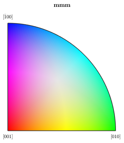
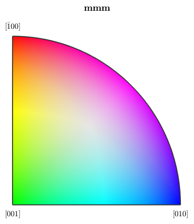
Obviously, the rotational angle is not a very distintive representative for orientations. A more common approach is to define a colorization of the fundamental secor of the inverse pole figure, a so called ipf color key, and to colorize orientations according to their position in a fixed inverse pole figure. Let's consider the following standard key.

% this defines an ipf color key for the Forsterite phase
ipfKey = ipfHSVKey(ebsd('Forsterite'))

% this is the colored fundamental sector
plot(ipfKey)

ipfKey = 
  ipfHSVKey with properties:

             colorPostRotation: [1×1 rotation]
               colorStretching: 1
                   whiteCenter: [1×1 vector3d]
                     grayValue: [0.2000 0.5000]
                  grayGradient: 0.5000
                      maxAngle: Inf
    inversePoleFigureDirection: [1×1 vector3d]
                        dirMap: [1×1 HSVDirectionKey]
                           CS1: [4×2 crystalSymmetry]
                           CS2: [1×1 specimenSymmetry]
                     antipodal: 0

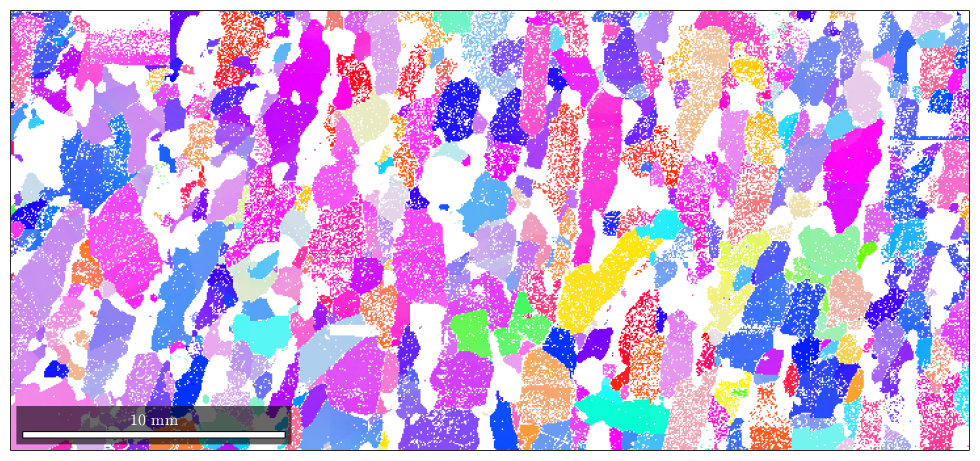
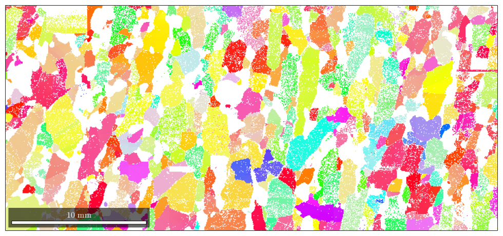
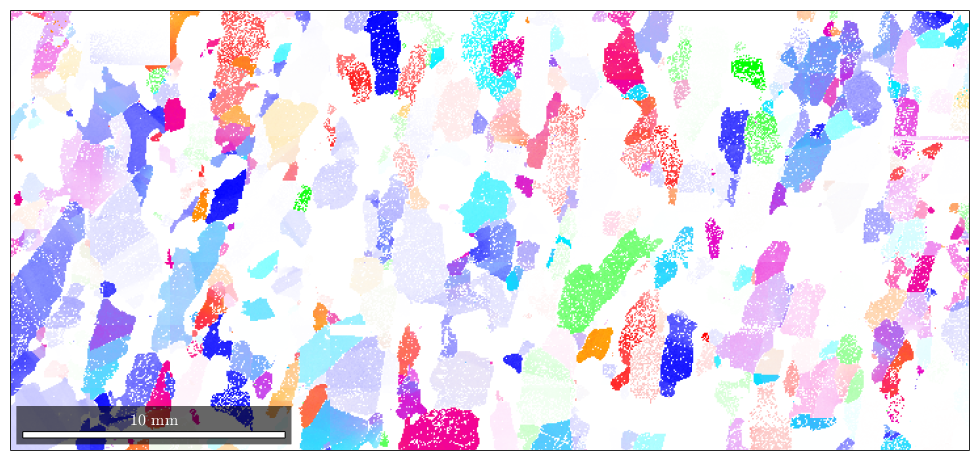
In order to apply this color key for colorizing the map we proceed as follows

% compute the colors
color = ipfKey.orientation2color(ebsd('Fo').orientations);

% plot the colors
close all
plot(ebsd('Forsterite'),color)

Orientation color key usually provide several options to alter the alignment of colors. Let's give some examples

% we may interchange green and blue by setting
ipfKey.colorPostRotation = reflection(yvector);

plot(ipfKey)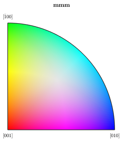

or cycle of colors red, green, blue by

ipfKey.colorPostRotation = rotation.byAxisAngle(zvector,120*degree);

plot(ipfKey)

Furthermore, we can explicitly set the inverse pole figure directions by

ipfKey.inversePoleFigureDirection = zvector;

% compute the colors again
color = ipfKey.orientation2color(ebsd('Forsterite').orientations);

% and plot them
close all
plot(ebsd('Forsterite'),color)

Besides the recommended color key ipfHSVKey MTEX includes a bunch of other color keys

Customizing the color

In some cases, it might be useful to color certain orientations after one needs. This can be done in two ways, either to color a certain fibre or a certain orientation.

Coloring certain fibres

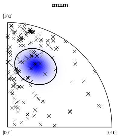
To color a fibre, one has to specify the crystal direction h together with its RGB color and the specimen direction r, which should be marked.

% define a fibre
f = fibre(Miller(1,1,1,csFo),zvector);

% set up coloring
ipfKey = ipfSpotKey(csFo);
ipfKey.inversePoleFigureDirection = f.r;
ipfKey.center = f.h;
ipfKey.color = [0 0 1];
ipfKey.psi = deLaValleePoussinKernel('halfwidth',7.5*degree);

plot(ebsd('fo'),ipfKey.orientation2color(ebsd('fo').orientations))

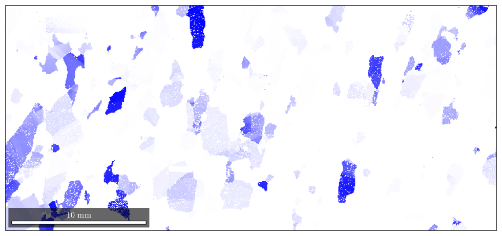
the option halfwidth controls half of the intensity of the color at a given distance. Here we have chosen the (111)[001] fibre to be drawn in blue, and at 7.5 degrees, where the blue should be only lighter.

plot(ipfKey)
hold on
circle(f.h.project2FundamentalRegion,15*degree,'linewidth',2)

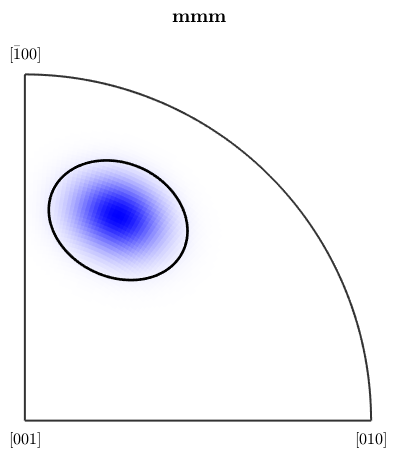
the percentage of blue colored area in the map is equivalent to the fibre volume

vol = volume(ebsd('fo').orientations,f,15*degree)

plotIPDF(ebsd('fo').orientations,zvector,'markercolor','k','marker','x','points',200)
hold off

vol =
    0.2480
  I'm plotting 200 random orientations out of 152345 given orientations

we can easily extend the colorcoding

% the centers in the inverse pole figure
ipfKey.center = Miller({0 0 1},{0 1 1},{1 1 1},{11 4 4},{5 0 2},{5 5 2},csFo);

% the correspnding collors
ipfKey.color = [[1 0 0];[0 1 0];[0 0 1];[1 0 1];[1 1 0];[0 1 1]];

% plot the key
plot(ipfKey)
hold on
plot(ebsd('fo').orientations,'MarkerFaceColor','none','MarkerEdgeColor','k','MarkerSize',3,'points',1000)
hold off

  I'm plotting 1000 random orientations out of 152345 given orientations

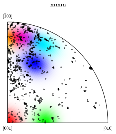
close all;
plot(ebsd('fo'),ipfKey.orientation2color(ebsd('fo').orientations))

Coloring certain orientations

We might be interested in locating some special orientation in our orientation map. The definition of colors for certain orientations is carried out similarly as in the case of fibres

ipfKey = spotColorKey(ebsd('Fo'));
ipfKey.center = mean(ebsd('Forsterite').orientations,'robust');
ipfKey.color = [0,0,1];
ipfKey.psi = deLaValleePoussinKernel('halfwidth',20*degree);

plot(ebsd('fo'),ipfKey.orientation2color(ebsd('fo').orientations))

% and the correspoding colormap
figure(2)
plot(ipfKey,'sections',9,'sigma')

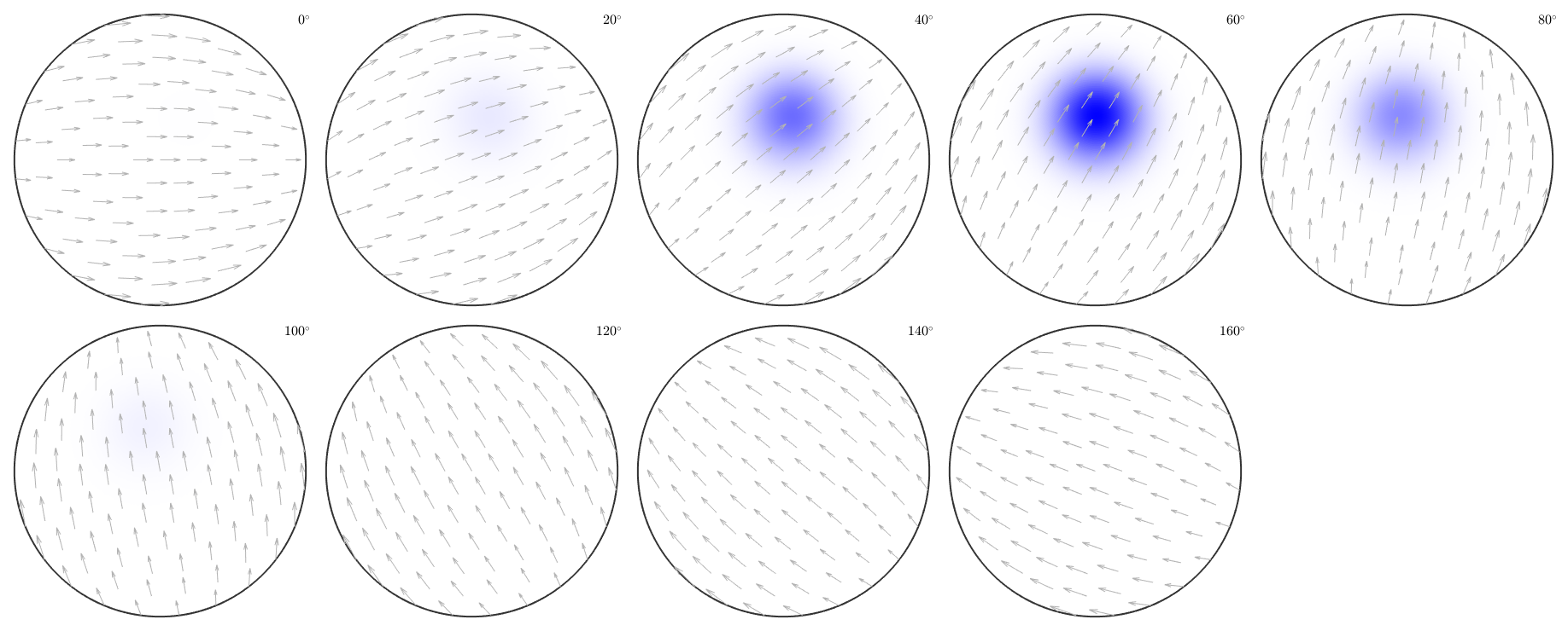
the area of the colored EBSD data in the map corresponds to the volume portion (in percent)

vol = 100 * volume(ebsd('fo').orientations,ipfKey.center,20*degree)

vol =
    1.3227

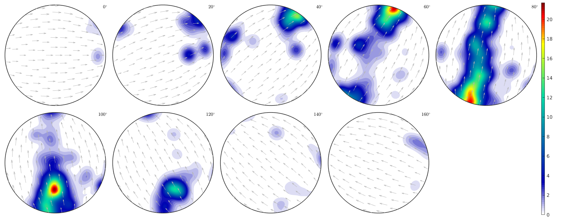
actually, the colored measurements stress a peak in the ODF

close all
odf = calcODF(ebsd('fo').orientations,'halfwidth',10*degree,'silent');
plot(odf,'sections',9,'silent','sigma')
mtexColorbar

Warning: Plot properties not compatible to previous plot! I'going to create a
new figure.

Combining different plots

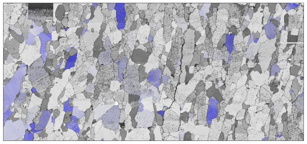
Combining different plots can be done either by plotting only subsets of the EBSD data or via the option 'faceAlpha'. Note that the option 'faceAlpha' requires the renderer of the figure to be set to 'opengl'.

close all;
plot(ebsd,ebsd.bc,'micronbar','off')
mtexColorMap black2white

ipfKey = ipfSpotKey(csFo);
ipfKey.inversePoleFigureDirection = zvector;
ipfKey.center = Miller(1,1,1,csFo);
ipfKey.color = [0 0 1];
ipfKey.psi = deLaValleePoussinKernel('halfwidth',7.5*degree);

hold on
plot(ebsd('fo'),ipfKey.orientation2color(ebsd('fo').orientations),'FaceAlpha',0.5)
hold off

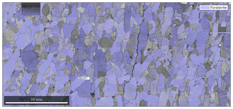
another example

close all;
plot(ebsd,ebsd.bc)
mtexColorMap black2white

hold on
plot(ebsd('fo'),'FaceAlpha',0.5)
hold off