Smoothing of EBSD Data
Discusses how to smooth and to fill missing values in EBSD data
Smoothing a single grain
Let's start out analysis by considering a single magnesium grain
% import standard data set
mtexdata twins

% compute grains
[grains,ebsd.grainId,ebsd.mis2mean] = calcGrains(ebsd,'angle',10*degree);

% restrict data to one single grain
[~,id] = max(grains.area);
oneGrain = grains(id);
ebsd = ebsd(oneGrain);

plot(ebsd,ebsd.orientations)

hold on
plot(oneGrain.boundary,'micronbar','off')
hold off
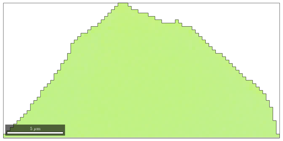
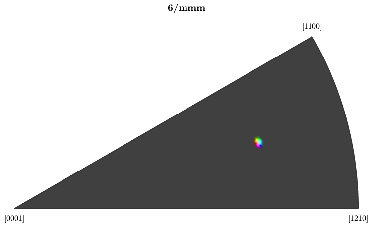
With the default colormap, we can not distinguish any orientation gradient within the grain. Let's adapt the colormap to this specific grain
ipfKey = ipfHSVKey(ebsd);

% set inversePoleFigureDirection  such that the mean orientation is
% colorized white
ipfKey.inversePoleFigureDirection = grains(id).meanOrientation * ipfKey.whiteCenter;

% concentrate the colors around the mean orientation
ipfKey.maxAngle = 1.5*degree;

% plot the colormap
plot(ipfKey,'resolution',0.25*degree)
Warning: Possibly applying an orientation to an object in specimen coordinates!
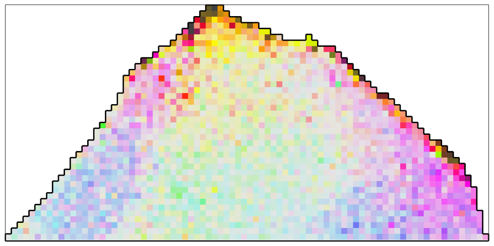
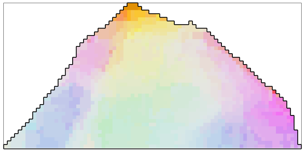
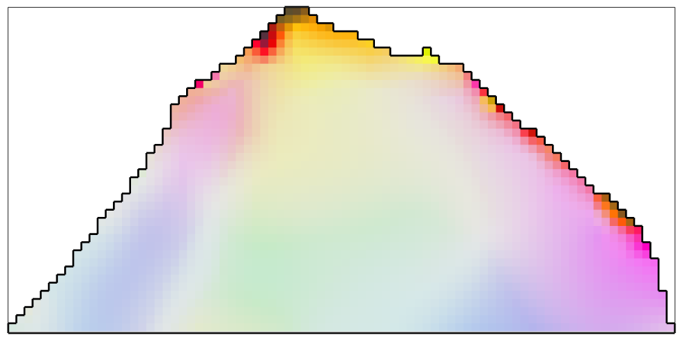
With the new colormap, we can clearly see the noise overlapping the texture gradient within the grain.
% plot the grain
plot(ebsd,ipfKey.orientation2color(ebsd.orientations),'micronbar','off')

hold on
plot(oneGrain.boundary,'linewidth',2)
hold off
The Mean Filter
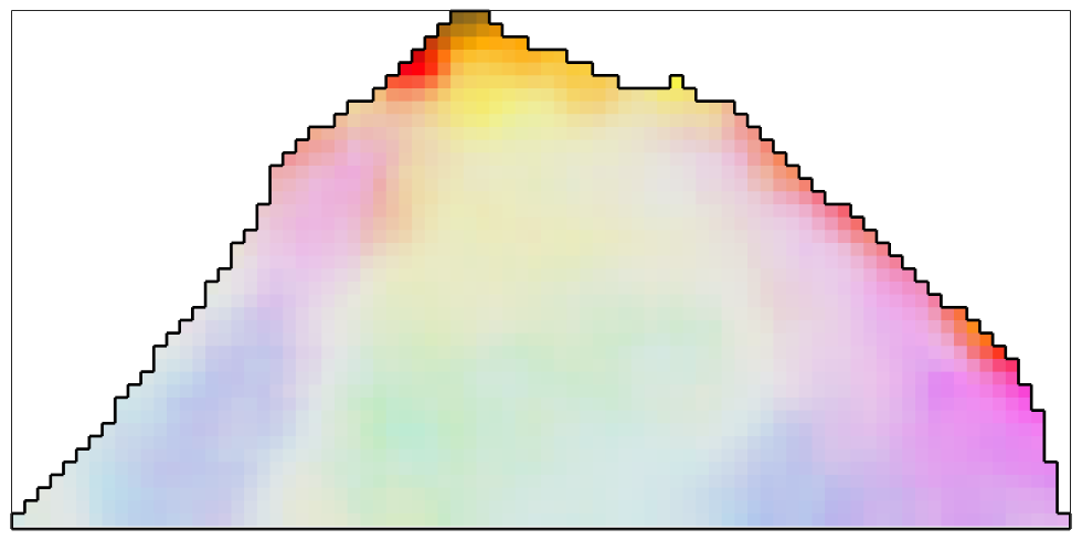
The simplest filter to apply to the orientation data is the meanFilter which simply takes the mean of all orientations within a certain neighborhood.
% define the meanFilter
F = meanFilter;

% smooth the data
ebsd_smoothed = smooth(ebsd,F);

% plot the smoothed data
plot(ebsd_smoothed('indexed'),...
  ipfKey.orientation2color(ebsd_smoothed('indexed').orientations),'micronbar','off')

hold on
plot(oneGrain.boundary,'linewidth',2)
hold off

As an additional option, one can specify the size of the neighborhood and weights for the averaging. Let's define a 5x5 window with weights coming from the Gaussian distribution.
[x,y] = meshgrid(-2:2);
F.weights = exp(-(x.^2+y.^2)/10);

% smooth the data
ebsd_smoothed = smooth(ebsd,F)

% plot the smoothed data
plot(ebsd_smoothed('indexed'),...
  ipfKey.orientation2color(ebsd_smoothed('indexed').orientations),'micronbar','off')

hold on
plot(oneGrain.boundary,'linewidth',2)
hold off
ebsd_smoothed = EBSD

 Phase  Orientations     Mineral       Color  Symmetry  Crystal reference frame
     0    1264 (39%)  notIndexed
     1    2016 (61%)   Magnesium  light blue     6/mmm       X||a*, Y||b, Z||c*

 Properties: bands, bc, bs, error, mad, x, y, grainId, mis2mean
 Scan unit : um
The Median Filter
The disadvantage of the mean filter is that is smoothes away all subgrain boundaries and is quite sensitive against outliers. A more robust filter which also preserves subgrain boundaries is the median filter
F = medianFilter;

% define the size of the window to be used for finding the median
F.numNeighbours = 3; % this corresponds to a 7x7 window

% smooth the data
ebsd_smoothed = smooth(ebsd,F);

% plot the smoothed data
plot(ebsd_smoothed('indexed'),...
  ipfKey.orientation2color(ebsd_smoothed('indexed').orientations),'micronbar','off')

hold on
plot(oneGrain.boundary,'linewidth',2)
hold off
The Kuwahara Filer
F = KuwaharaFilter;
F.numNeighbours = 5;

% smooth the data
ebsd_smoothed = smooth(ebsd,F);

% plot the smoothed data
plot(ebsd_smoothed('indexed'),...
  ipfKey.orientation2color(ebsd_smoothed('indexed').orientations),'micronbar','off')

hold on
plot(oneGrain.boundary,'linewidth',2)
hold off
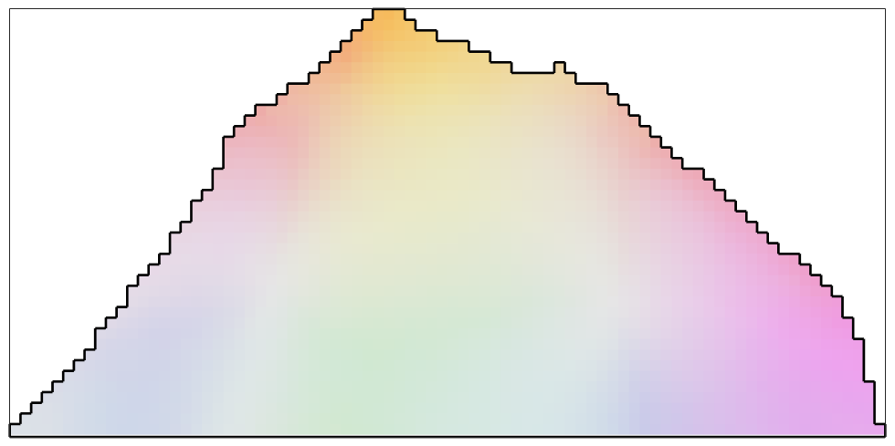
The Smoothing Spline Filter
The smoothing spline filter is up to now the only filter that automatically calibrates the smoothing parameter
F = splineFilter;

% smooth the data
ebsd_smoothed = smooth(ebsd,F);

% plot the smoothed data
plot(ebsd_smoothed('indexed'),...
  ipfKey.orientation2color(ebsd_smoothed('indexed').orientations),'micronbar','off')

hold on
plot(oneGrain.boundary,'linewidth',2)
hold off

% the smoothing parameter determined during smoothing is
F.alpha
ans =
    4.6123
The halfquadratic Filter
The halfquadratic filter differs from the smoothing spline filter by the fact that it better preserves inner grain boundaries. We will see this in a later example.
F = halfQuadraticFilter;
F.alpha = 0.25; %set the smoothing parameter

% smooth the data
ebsd_smoothed = smooth(ebsd,F);

% plot the smoothed data
plot(ebsd_smoothed('indexed'),...
  ipfKey.orientation2color(ebsd_smoothed('indexed').orientations),'micronbar','off')

hold on
plot(oneGrain.boundary,'linewidth',2)
hold off
The Infimal Convolution Filter
The infimal convolution filter differs from the smoothing spline filter by the fact that it better preserves inner grain boundaries. We will see this in a later example.
F = infimalConvolutionFilter;
F.lambda = 0.01; %smoothing parameter for the gradient
F.mu = 0.005;% smoothing parameter for the hessian

% smooth the data
ebsd_smoothed = smooth(ebsd,F);

% plot the smoothed data
plot(ebsd_smoothed('indexed'),...
  ipfKey.orientation2color(ebsd_smoothed('indexed').orientations),'micronbar','off')

hold on
plot(oneGrain.boundary,'linewidth',2)
hold off
Interpolating Missing Data
The filters above can also be used to interpolate missindexed orientations.
A synthetic example
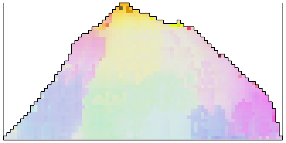
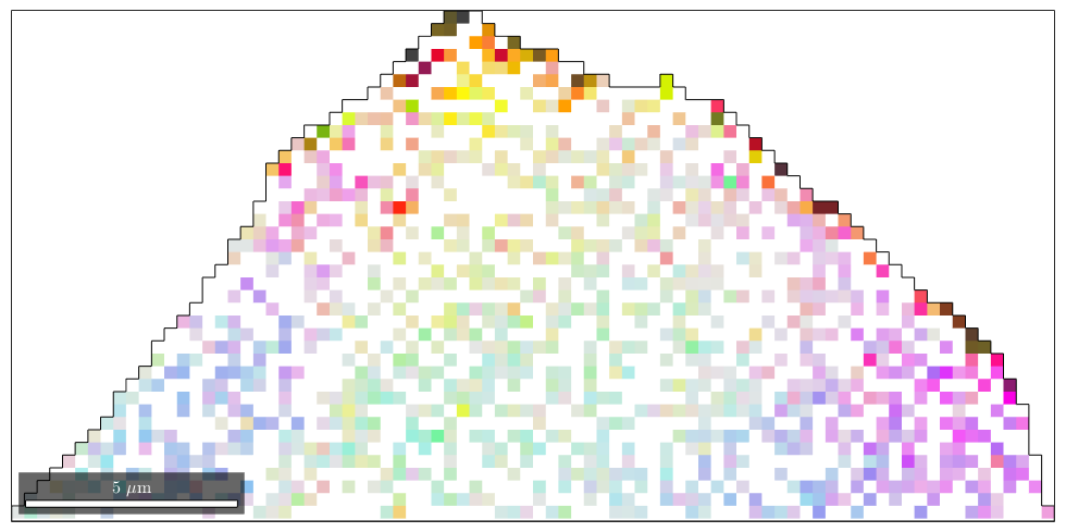
In the following example, we randomly set 50 percent of the measured orientations to nan.
ebsdNaN = ebsd;

% set 50 percent of the orientations to nan
ind = discretesample(length(ebsd),round(length(ebsd)*50/100));
ebsdNaN(ind).orientations = orientation.nan(ebsd.CS);

% plot the reduced data
plot(ebsdNaN,ipfKey.orientation2color(ebsdNaN.orientations))
hold on
plot(oneGrain.boundary,'micronbar','off')
hold off
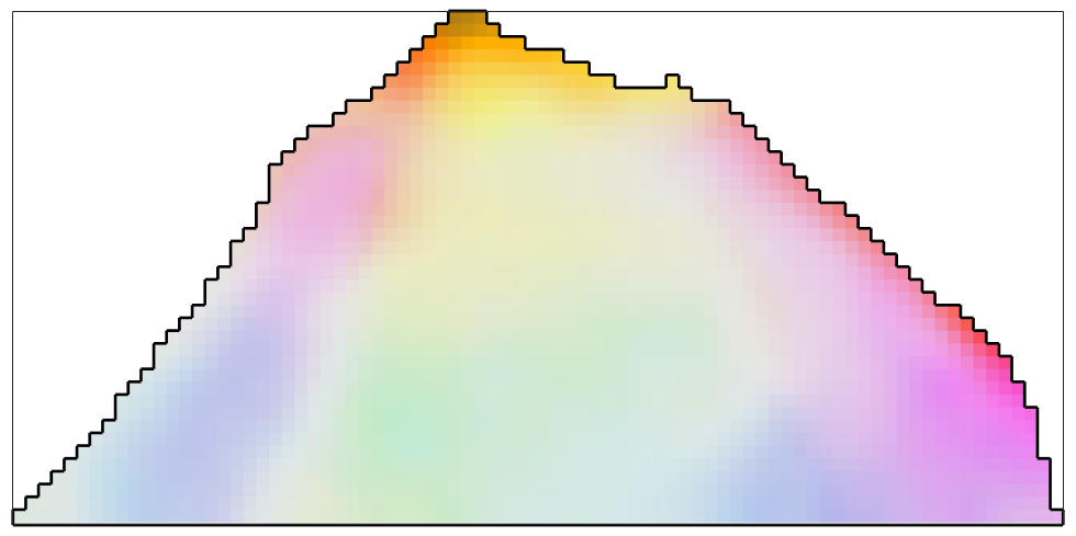
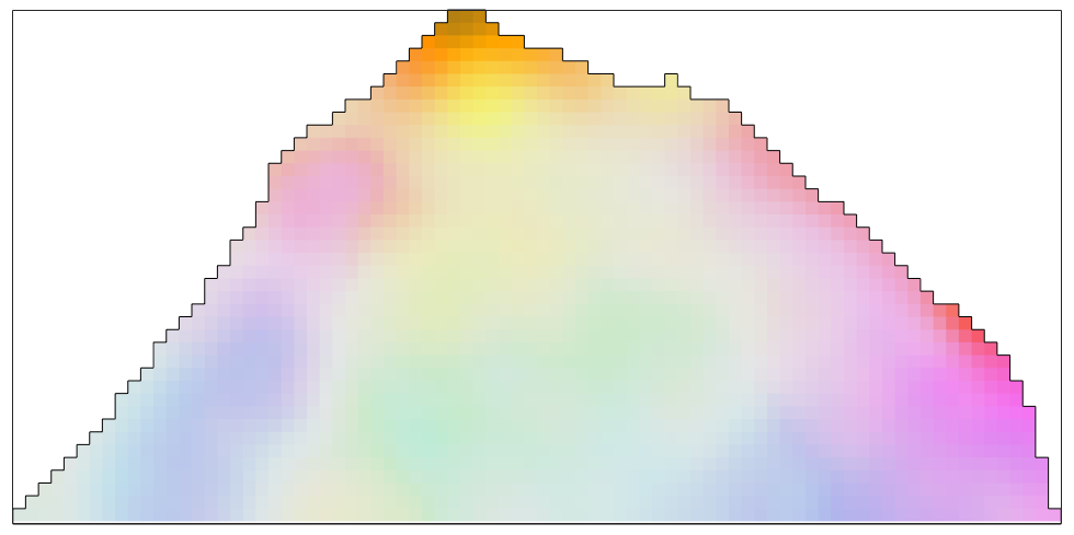
By default, all orientations that are set to nan are interpolated.
% interpolate the missing data with the smoothing spline filter
ebsdNaN_smoothed = smooth(ebsdNaN,splineFilter);
color = ipfKey.orientation2color(ebsdNaN_smoothed('indexed').orientations);
plot(ebsdNaN_smoothed('indexed'),color,'micronbar','off')
hold on
plot(oneGrain.boundary)
hold off
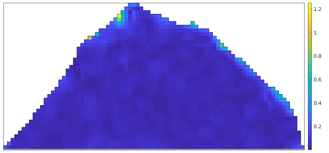
We may plot the misorientation angle between the interpolated orientations and the measured orientations
omega = angle(ebsdNaN_smoothed('indexed').orientations, ...
  ebsd_smoothed('indexed').orientations);
plot(ebsd_smoothed('indexed'),omega./degree,'micronbar','off')
mtexColorbar

hold on
plot(oneGrain.boundary)
hold off
A real world example
Let's consider a subset of the
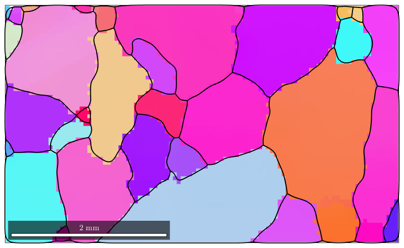
close all; plotx2east
mtexdata forsterite
ebsd = ebsd(inpolygon(ebsd,[10 4 5 3]*10^3));
plot(ebsd('Fo'),ebsd('Fo').orientations)
hold on
plot(ebsd('En'),ebsd('En').orientations)
plot(ebsd('Di'),ebsd('Di').orientations)

% compute grains
[grains,ebsd.grainId] = calcGrains(ebsd('indexed'),'angle',10*degree);


% remove small grains
ebsd(grains(grains.grainSize < 3)) = [];

% and repeat the grain computation
[grains,ebsd.grainId] = calcGrains(ebsd('indexed'),'angle',10*degree);

%
grains = smooth(grains,5);

% plot the boundary of all grains
plot(grains.boundary,'linewidth',2)
hold off
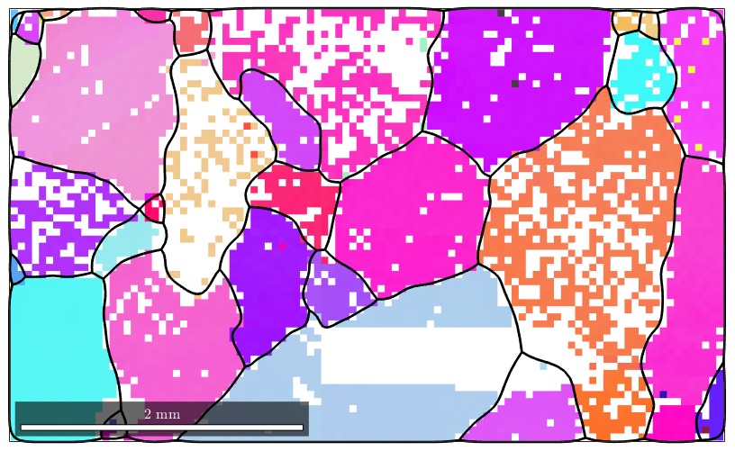
Using the option fill the command smooth fills the holes inside the grains. Note that the nonindexed pixels at the grain boundaries kept untouched. In order to allow MTEX to decide whether a pixel is inside a grain or not, the grain variable has to be passed as an additional argument.
F = halfQuadraticFilter;
F.alpha = 0.01;
F.eps = 0.001;
ebsd_smoothed = smooth(ebsd('indexed'),F,'fill',grains);

plot(ebsd_smoothed('Fo'),ebsd_smoothed('Fo').orientations)
hold on
plot(ebsd_smoothed('En'),ebsd_smoothed('En').orientations)
plot(ebsd_smoothed('Di'),ebsd_smoothed('Di').orientations)

% plot the boundary of all grains
plot(grains.boundary,'linewidth',1.5)

% stop overide mode
hold off
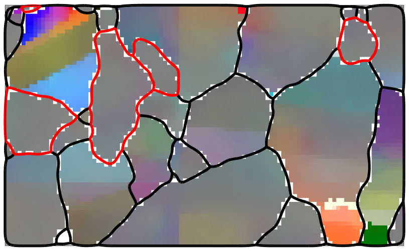
In order to visualize the orientation gradient within the grains, we plot the misorientation to the meanorientation. We observe that the mis2mean varies smoothly also within the regions of not indexed orientations.
% plot mis2mean for all phases
ipfKey = axisAngleColorKey(ebsd_smoothed('Fo'));
ipfKey.oriRef = grains(ebsd_smoothed('fo').grainId).meanOrientation;
ipfKey.maxAngle = 2.5*degree;

color = ipfKey.orientation2color(ebsd_smoothed('Fo').orientations);
plot(ebsd_smoothed('Fo'),color,'micronbar','off')

hold on
ipfKey.oriRef = grains(ebsd_smoothed('En').grainId).meanOrientation;

plot(ebsd_smoothed('En'),ipfKey.orientation2color(ebsd_smoothed('En').orientations))


% plot boundary
plot(grains.boundary,'linewidth',4)
plot(grains('En').boundary,'lineWidth',4,'lineColor','r')
hold off
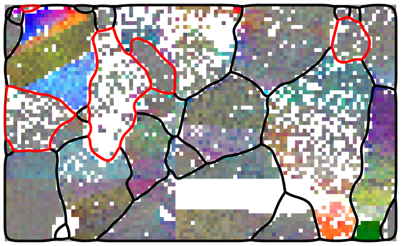
For comparison
ipfKey.oriRef = grains(ebsd('fo').grainId).meanOrientation;
ipfKey.maxAngle = 2.5*degree;

color = ipfKey.orientation2color(ebsd('Fo').orientations);
plot(ebsd('Fo'),color,'micronbar','off')

hold on
ipfKey.oriRef = grains(ebsd('En').grainId).meanOrientation;

plot(ebsd('En'),ipfKey.orientation2color(ebsd('En').orientations))


% plot boundary
plot(grains.boundary,'linewidth',4)
plot(grains('En').boundary,'lineWidth',4,'lineColor','r')
hold off
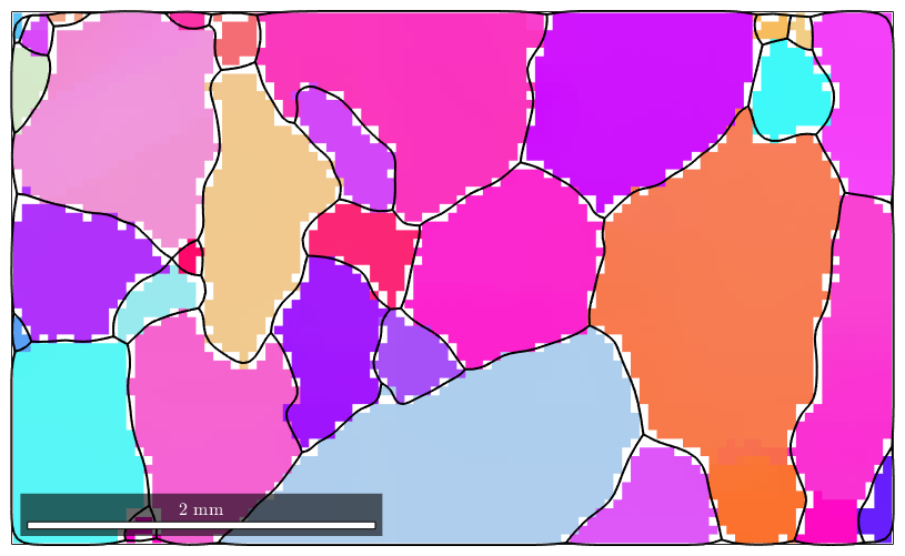
If no grain variable is passed to the smoothing command the not indexed pixels are assigned to the nearest neighbor.
ebsd_smoothed = smooth(ebsd('indexed'),F,'fill');

plot(ebsd_smoothed('Fo'),ebsd_smoothed('Fo').orientations)
hold on
plot(ebsd_smoothed('En'),ebsd_smoothed('En').orientations)
plot(ebsd_smoothed('Di'),ebsd_smoothed('Di').orientations)

% plot the boundary of all grains
plot(grains.boundary,'linewidth',1.5)

% stop overide mode
hold off
| DocHelp 0.1 beta |