Visualizing EBSD data with sharp textures
How visualize texture gradients within grains
| On this page ... |
| Sharpening the default colorcoding |
Using advanced color keys is particularly useful when visualizing sharp data. Let us consider the following calcite data set
% plotting conventions
plotx2east, plotb2east
mtexdata sharp

ebsd = ebsd('calcite');

ipfKey = ipfColorKey(ebsd);

close all;
plot(ebsd,ipfKey.orientation2color(ebsd.orientations))
 loading data ...
 saving data to /home/hielscher/mtex/master/data/sharp.mat

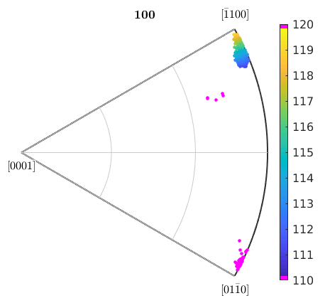
and have a look into the 100 inverse pole figure.
% compute the positions in the inverse pole figure
h = ebsd.orientations .\ vector3d.X;
h = project2FundamentalRegion(h);

% compute the azimuth angle in degree
color = h.rho ./ degree;

plotIPDF(ebsd.orientations,vector3d.X,'property',color,'MarkerSize',3,'grid')
mtexColorbar
I'm plotting 8333 random orientations out of 20119 given orientations

We see that all individual orientations are clustered around azimuth angle 115 degrees with some outliers at 125 and 130 degree. In order to increase the contrast for the main group, we restrict the color range from 110 degree to 120 degree.
caxis([110 120]);

% by the following lines we colorcode the outliers in purple.
cmap = colormap;
cmap(end,:) = [1 0 1]; % make last color purple
cmap(1,:) = [1 0 1];   % make first color purple
colormap(cmap)
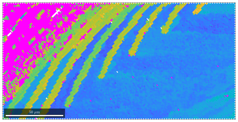
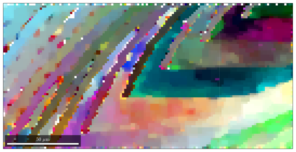
The same colorcoding we can now apply to the EBSD map.
% plot the data with the customized color
plot(ebsd,color)

% set scaling of the angles to 110 - 120 degree
caxis([110 120]);

% colorize outliers in purple.
cmap = colormap;
cmap(end,:) = [1 0 1];
cmap(1,:) = [1 0 1];
colormap(cmap)
Sharpening the default colorcoding
Next, we want to apply the same ideas as above to the default MTEX color key, i.e. we want to stretch the colors such that they cover just the orientations of interest.
ipfKey = ipfHSVKey(ebsd.CS.properGroup);

% To this end, we first compute the inverse pole figure direction such that
% the mean orientation is just at the gray spot of the inverse pole figure
ipfKey.inversePoleFigureDirection = mean(ebsd.orientations,'robust') * ipfKey.whiteCenter;

close all;
plot(ebsd,ipfKey.orientation2color(ebsd.orientations))
Warning: Possibly applying an orientation to an object in specimen coordinates!

We observe that the orientation map is almost completely gray, except for the outliers which appears black. Next, we use the option maxAngle to increase contrast in the grayish part
ipfKey.maxAngle = 7.5*degree;
plot(ebsd,ipfKey.orientation2color(ebsd.orientations))
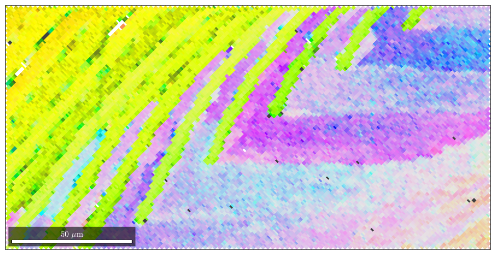
You may play around with the option maxAngle to obtain better results. As for interpretation keep in mind that white color represents the mean orientation and the color becomes more saturated and later dark as the orientation to color diverges from the mean orientation.
Let's have a look at the corresponding color map.
plot(ipfKey,'resolution',0.25*degree)

% plot orientations into the color key
hold on
plotIPDF(ebsd.orientations,'points',10,'MarkerSize',1,'MarkerFaceColor','w','MarkerEdgeColor','w')
hold off
I'm plotting 10 random orientations out of 20119 given orientations

observe how in the inverse pole figure the orientations are scattered closely around the white center. Together with the fact that the transition from white to color is quite rapidly, this gives a high contrast.
[grains,ebsd.grainId] = calcGrains(ebsd,'angle',1.5*degree);
ebsd(grains(grains.grainSize<=3)) = [];
[grains,ebsd.grainId] = calcGrains(ebsd,'angle',1.5*degree);

grains = smooth(grains,5);
ipfKey = axisAngleColorKey(ebsd('indexed'));

% use for the reference orientation the grain mean orientation
ipfKey.oriRef = grains.meanOrientation(ebsd.grainId);

plot(ebsd,ipfKey.orientation2color(ebsd.orientations))

hold on
plot(grains.boundary,'lineWidth',4)
hold off
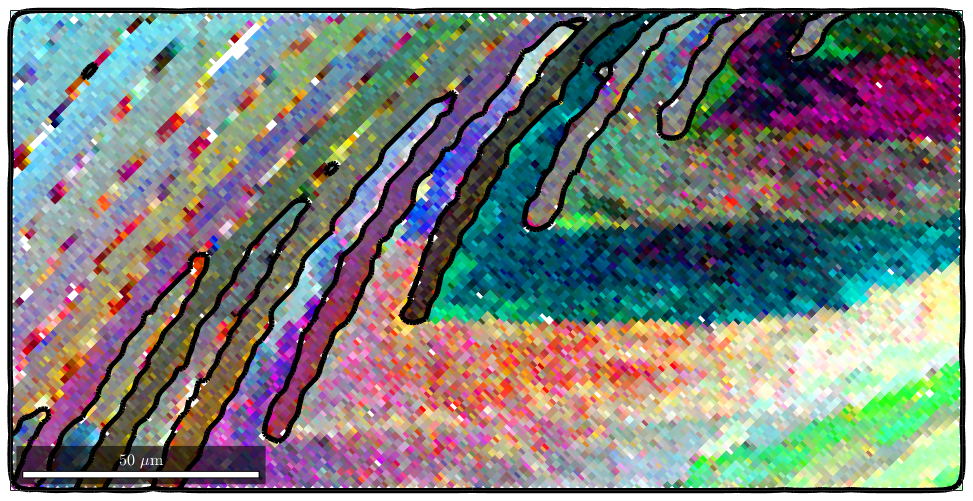
F = halfQuadraticFilter;
F.alpha = 0.01;
F.eps = 1e-6;
F.tol = 1e-10;

ebsdS = smooth(ebsd,F);

% use for the reference orientation the grain mean orientation
ipfKey.oriRef = grains.meanOrientation(ebsdS('indexed').grainId);

plot(ebsdS('indexed'),ipfKey.orientation2color(ebsdS('indexed').orientations))

%hold on
%plot(grains.boundary,'lineWidth',4)
%hold off
F = infimalConvolutionFilter;
F.lambda = 0.01;
F.mu = 0.02;

ebsdS = smooth(ebsd,F);

[grains,ebsdS.grainId] = calcGrains(ebsdS,'angle',1*degree);
%ebsdS(grains(grains.grainSize<=3)) = [];
%[grains,ebsdS.grainId] = calcGrains(ebsdS,'angle',1.5*degree);

grains = smooth(grains,5);


% use for the reference orientation the grain mean orientation
ipfKey.oriRef = grains(ebsdS('indexed').grainId).meanOrientation;
%ipfKey.oriRef = mean(ebsdS('indexed').orientations);

plot(ebsdS('indexed'),ipfKey.orientation2color(ebsdS('indexed').orientations),'micronbar','off')

hold on
plot(grains.boundary,'lineWidth',4)
hold off

Another example is when analyzing the orientation distribution within grains
mtexdata forsterite
ebsd = ebsd('indexed');

% segment grains
[grains,ebsd.grainId] = calcGrains(ebsd);

% find largest grains
largeGrains = grains(grains.grainSize > 800)

ebsd = ebsd(largeGrains(1))
largeGrains = grain2d

 Phase  Grains  Pixels     Mineral  Symmetry  Crystal reference frame
     1      56   85514  Forsterite       mmm
     2       2    1969   Enstatite       mmm

 boundary segments: 17507
 triple points: 1247

 Properties: GOS, meanRotation


ebsd = EBSD

 Phase  Orientations     Mineral       Color  Symmetry  Crystal reference frame
     1   1453 (100%)  Forsterite  light blue       mmm

 Properties: bands, bc, bs, error, mad, x, y, grainId
 Scan unit : um
When plotting one specific grain with its orientations we see that they all are very similar and, hence, get the same color
% plot a grain
close all
plot(largeGrains(1).boundary,'linewidth',2)
hold on
plot(ebsd,ebsd.orientations)
hold off

when applying the option sharp MTEX colors the mean orientation as white and scales the maximum saturation to fit the maximum misorientation angle. This way deviations of the orientation within one grain can be visualized.
% plot a grain
plot(largeGrains(1).boundary,'linewidth',2)
hold on
ipfKey = ipfHSVKey(ebsd);
ipfKey.inversePoleFigureDirection = mean(ebsd.orientations) * ipfKey.whiteCenter;
ipfKey.maxAngle = 2*degree;
plot(ebsd,ipfKey.orientation2color(ebsd.orientations))
hold off
Warning: Possibly applying an orientation to an object in specimen coordinates!

| DocHelp 0.1 beta |