Bingham distribution and EBSD data
testing rotational symmetry of individual orientations
| On this page ... |
| Bingham Distribution |
| The bipolar case and unimodal distribution |
| Prolate case and fibre distribution |
| Oblate case |
Bingham Distribution
The quaternionic Bingham distribution has the density
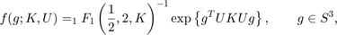
where  are an
  orthogonal matrix with unit quaternions
  in the column and
  a diagonal matrix with the entries
  describing the shape of the distribution.
  is the hypergeometric function with matrix argument normalizing the density.
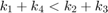
The shape parameters 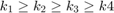 give
give
- a bipolar distribution, if
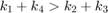 ,
,
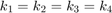
- a circular distribution, if
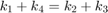 ,
,
- a spherical distribution, if
 ,
,
- a uniform distribution, if
 ,
,
in unit quaternion space. Since the quaternion +g and -g describes the same rotation, the bipolar distribution corresponds to an unimodal distribution in orientation space. Moreover, we would call the circular distribution a fibre in orientation space.
The general setup of the Bingham distribution in MTEX is done as follows
cs = crystalSymmetry('1');

kappa = [100 90 80 0];   % shape parameters
U     = eye(4);          % orthogonal matrix

odf = BinghamODF(kappa,U,cs)
odf = ODF
  crystal symmetry : 1, X||a, Y||b*, Z||c*
  specimen symmetry: 1

  Bingham portion:
     kappa: 100 90 80 0
    weight: 1
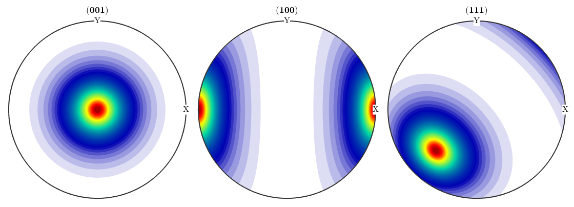
h = [Miller(0,0,1,cs) Miller(1,0,0,cs) Miller(1,1,1,cs)];
plotPDF(odf,h,'antipodal','silent');


% plot(odf,'sections',10)
The bipolar case and unimodal distribution
First, we define some unimodal odf
odf_spherical = unimodalODF(orientation.id(cs),'halfwidth',20*degree)
odf_spherical = ODF
  crystal symmetry : 1, X||a, Y||b*, Z||c*
  specimen symmetry: 1

  Radially symmetric portion:
    kernel: de la Vallee Poussin, halfwidth 20°
    center: (0°,0°,0°)
    weight: 1
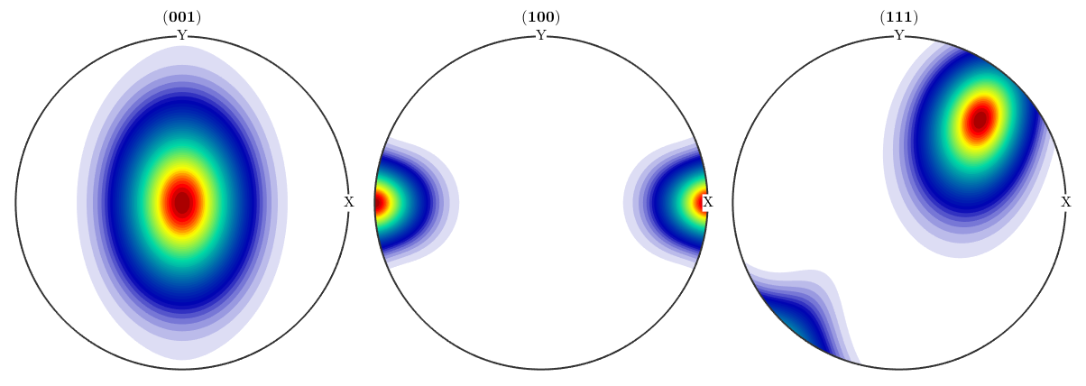
plotPDF(odf_spherical,h,'antipodal','silent')
Next, we simulate individual orientations from this odf, in a scattered axis/angle plot in which the simulated data looks like a sphere
ori_spherical = calcOrientations(odf_spherical,1000);
close all
scatter(ori_spherical)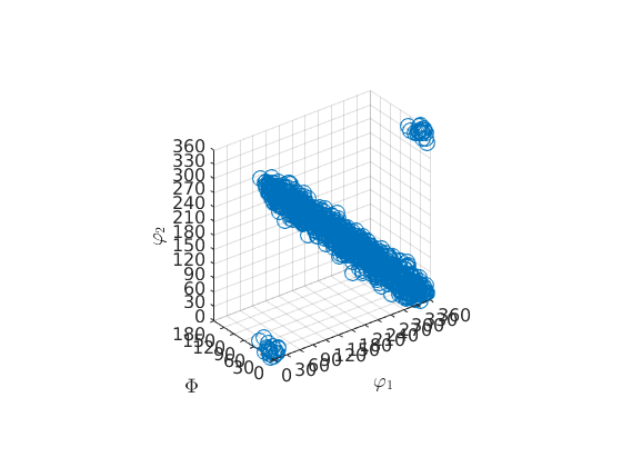
From this simulated EBSD data, we can estimate the parameters of the Bingham distribution,
calcBinghamODF(ori_spherical)
ans = ODF
  crystal symmetry : 1, X||a, Y||b*, Z||c*
  specimen symmetry: 1

  Bingham portion:
     kappa: 0 0.82596 2.8101 26.7107
    weight: 1
where U is the orthogonal matrix of eigenvectors of the orientation tensor and kappa the shape parameters associated with the U.
next, we test the different cases of the distribution on rejection
T_spherical = bingham_test(ori_spherical,'spherical','approximated');
T_oblate    = bingham_test(ori_spherical,'prolate',  'approximated');
T_prolate   = bingham_test(ori_spherical,'oblate',   'approximated');

t = [T_spherical T_oblate T_prolate]
t =
    0.3441    0.1160    0.5486
The spherical test case failed to reject it for some level of significance, hence we would dismiss the hypothesis prolate and oblate.
odf_spherical = BinghamODF(kappa,U,crystalSymmetry,specimenSymmetry)
odf_spherical = ODF
  crystal symmetry : 1, X||a, Y||b*, Z||c*
  specimen symmetry: 1

  Bingham portion:
     kappa: 100 90 80 0
    weight: 1
plotPDF(odf_spherical,h,'antipodal','silent')

Prolate case and fibre distribution
The prolate case correspondes to a fibre.
odf_prolate = fibreODF(Miller(0,0,1,crystalSymmetry('1')),zvector,...
  'halfwidth',20*degree)
odf_prolate = ODF
  crystal symmetry : 1, X||a, Y||b*, Z||c*
  specimen symmetry: 1

  Fibre symmetric portion:
    kernel: de la Vallee Poussin, halfwidth 20°
    fibre: (001) - 0,0,1
    weight: 1
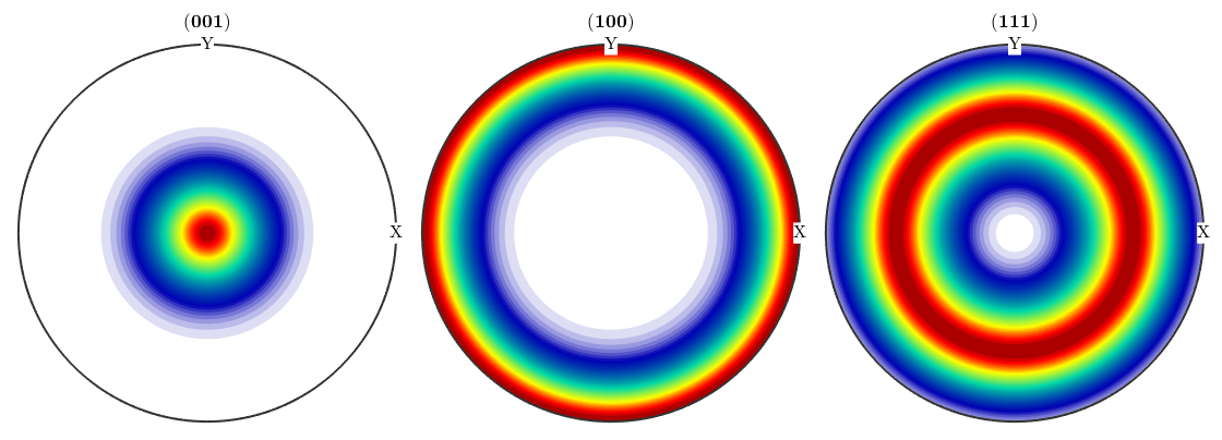
plotPDF(odf_prolate,h,'upper','silent')
As before, we generate some random orientations from a model odf. The shape in an axis/angle scatter plot reminds of a cigar
ori_prolate = calcOrientations(odf_prolate,1000);
close all
scatter(ori_prolate)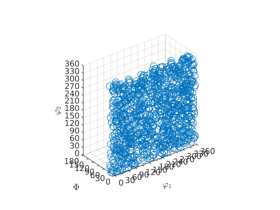
We estimate the parameters of the Bingham distribution
calcBinghamODF(ori_prolate)
ans = ODF
  crystal symmetry : 1, X||a, Y||b*, Z||c*
  specimen symmetry: 1

  Bingham portion:
     kappa: 0 2.2873 51.2566 52.282
    weight: 1
and test on the three cases
T_spherical = bingham_test(ori_prolate,'spherical','approximated');
T_oblate    = bingham_test(ori_prolate,'prolate',  'approximated');
T_prolate   = bingham_test(ori_prolate,'oblate',   'approximated');

t = [T_spherical T_oblate T_prolate]
t =
    1.0000    0.2213    1.0000
The test clearly rejects the spherical and prolate case, but not the prolate. We construct the Bingham distribution from the parameters, it might show some skewness
odf_prolate = BinghamODF(kappa,U,crystalSymmetry,specimenSymmetry)
odf_prolate = ODF
  crystal symmetry : 1, X||a, Y||b*, Z||c*
  specimen symmetry: 1

  Bingham portion:
     kappa: 100 90 80 0
    weight: 1
plotPDF(odf_prolate,h,'antipodal','silent')
Oblate case
The oblate case of the Bingham distribution has no direct counterpart in terms of texture components, thus we can construct it straightforward
odf_oblate = BinghamODF([50 50 50 0],eye(4),crystalSymmetry,specimenSymmetry)
odf_oblate = ODF
  crystal symmetry : 1, X||a, Y||b*, Z||c*
  specimen symmetry: 1

  Bingham portion:
     kappa: 50 50 50 0
    weight: 1
plotPDF(odf_oblate,h,'antipodal','silent')
The oblate cases in axis/angle space remind on a disk
ori_oblate = calcOrientations(odf_oblate,1000);
close all
scatter(ori_oblate)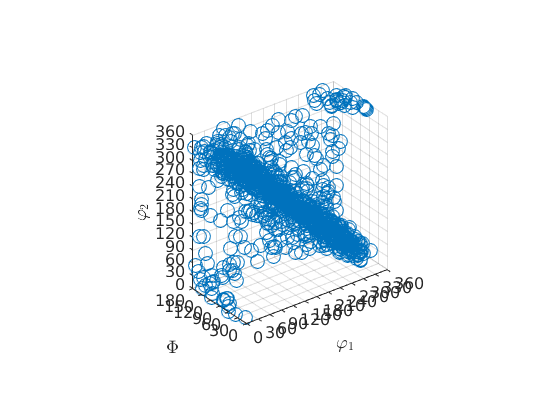
We estimate the parameters again
calcBinghamODF(ori_oblate)
ans = ODF
  crystal symmetry : 1, X||a, Y||b*, Z||c*
  specimen symmetry: 1

  Bingham portion:
     kappa: 0 45.8815 45.9351 47.454
    weight: 1
and do the tests
T_spherical = bingham_test(ori_oblate,'spherical','approximated');
T_oblate    = bingham_test(ori_oblate,'prolate',  'approximated');
T_prolate   = bingham_test(ori_oblate,'oblate',   'approximated');

t = [T_spherical T_oblate T_prolate]
t =
    1.0000    1.0000    0.1396
the spherical and oblate case are clearly rejected, the prolate case failed to reject for some level of significance
odf_oblate = BinghamODF(kappa, U,crystalSymmetry,specimenSymmetry)
odf_oblate = ODF
  crystal symmetry : 1, X||a, Y||b*, Z||c*
  specimen symmetry: 1

  Bingham portion:
     kappa: 100 90 80 0
    weight: 1
plotPDF(odf_oblate,h,'antipodal','silent')

| DocHelp 0.1 beta |