Pole Figure Color Coding

A central issue when interpreting plots is to have a consistent color coding among all plots. In MTEX this can be achieved in two ways. If the minimum and maximum values are known then one can specify the color range directly using the options colorrange or contourf, or the command setcolorrange is used which allows setting the color range afterward.

A sample ODFs and Simulated Pole Figure Data

Let us first define some model ODF_index.html ODFs> to be plotted later on.

cs = crystalSymmetry('-3m');
odf = fibreODF(Miller(1,1,0,cs),zvector)
pf = calcPoleFigure(odf,[Miller(1,0,0,cs),Miller(1,1,1,cs)],...
  equispacedS2Grid('points',500,'antipodal'));

 
odf = ODF  
  crystal symmetry : -3m1, X||a*, Y||b, Z||c*
  specimen symmetry: 1
 
  Fibre symmetric portion:
    kernel: de la Vallee Poussin, halfwidth 10°
    fibre: (11-20) - 0,0,1
    weight: 1
 

Back to Top

Setting a Colormap

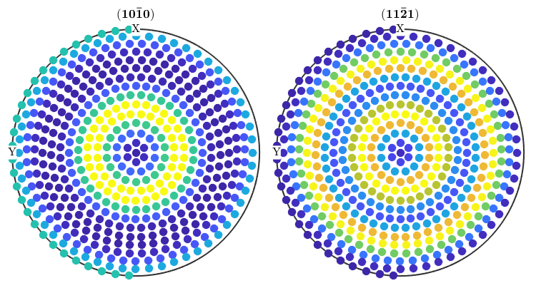
By default, MTEX uses the default MATLAB colormap jet, which varies from blue to red for increasing values.

plot(pf)

However, sometimes more simple colormaps are preferred, like the LaboTeX colormap

mtexColorMap LaboTeX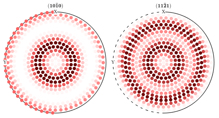

or a gray scale colormap.

mtexColorMap white2black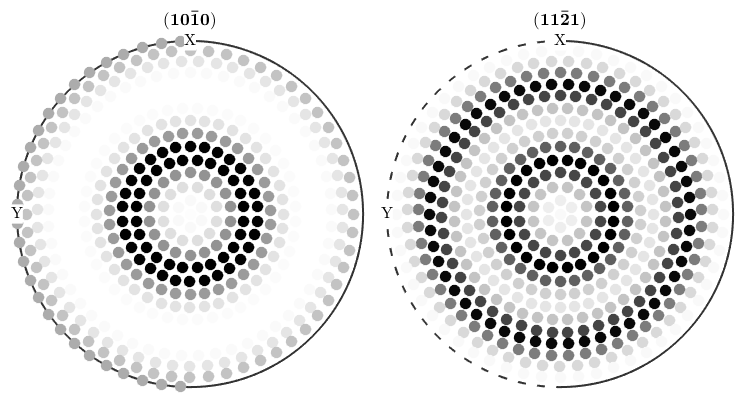

One can set a default colormap adding the following command to the configuration file mtex_settings.m

setMTEXpref('defaultColorMap',LaboTeXColorMap);

Back to Top

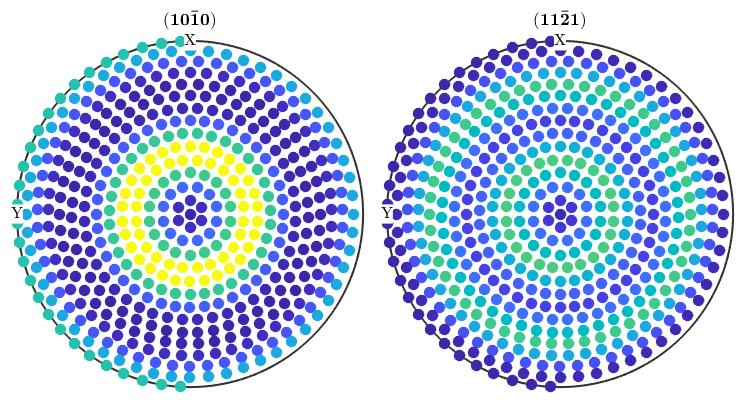
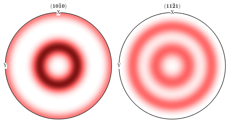
Tight Colorcoding

When the plot is called without any other option, the chosen color coding is the one called tight, which ranges the data independently from the other plots, i.e., for each subplot the largest value is assigned to the maximum color and the smallest value is assigned to the minimum color from the colormap.

close all
plot(pf)

Back to Top

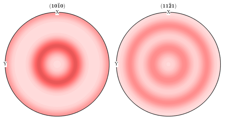
Equal Colorcoding

The tight colorcoding makes the reading and comparison between pole figures hard. If you want to have one colorcoding for all plots within one figure use the option colorrange to equal.

plot(pf,'colorrange','equal')

Back to Top

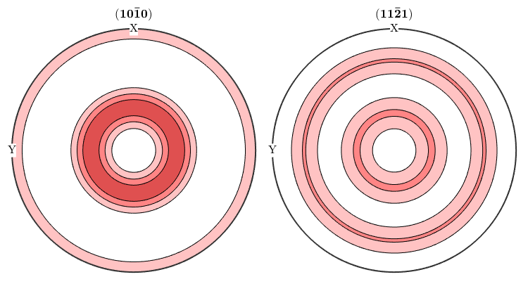
Setting an Explicit Colorrange

If you want to have a unified colorcoding for several figures you can set the colorrange directly in the plot command

close all
plotPDF(odf,[Miller(1,0,0,cs),Miller(1,1,1,cs)],...
  'colorrange',[0 4],'antipodal');
figure
plotPDF(.5*odf+.5*uniformODF(cs),[Miller(1,0,0,cs),Miller(1,1,1,cs)],...
  'colorrange',[0 4],'antipodal');

Back to Top

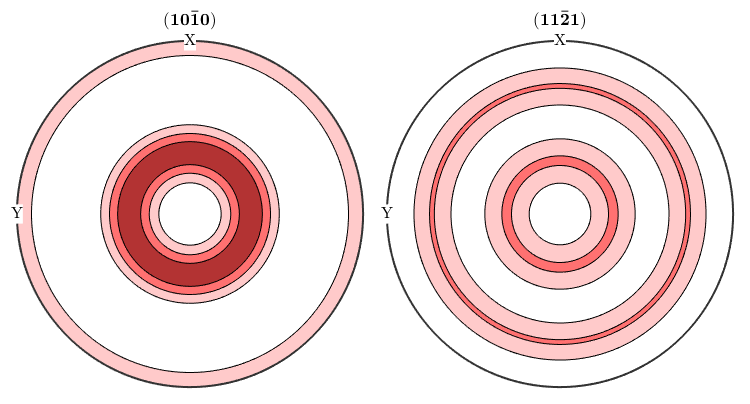
Setting the Contour Levels

In the case of contoured plots, you can also specify the contour levels directly

close all
plotPDF(odf,[Miller(1,0,0,cs),Miller(1,1,1,cs)],...
  'contourf',0:1:5,'antipodal')

Back to Top

Modifying the Color range After Plotting

The color range of the figures can also be adjusted afterward using the command setcolorrange

CLim(gcm,[0.38,3.9])

Back to Top

Logarithmic Plots

Sometimes logarithmic scaled plots are of interest. For this case all plots in MTEX understand the option logarithmic, e.g. TODO:

%close all;
%plotPDF(odf,[Miller(1,0,0,cs),Miller(1,1,1,cs)],'antipodal','logarithmic')
%setcolorrange([0.01 12]);
%mtexColorbar

Finally, lets set back the default colormap.

setMTEXpref('defaultColorMap',WhiteJetColorMap);

Back to Top

DocHelp 0.1 beta