EBSD Color Coding
Explains EBSD color coding.
| On this page ... |
| Colorcoding of orientations |
| Assigning the Euler angles to the RGB values |
| Colorcoding according to inverse pole figure |
See also
EBSD/plotspatial, grain/plotGrains, ebsdColorbar, orientation2color
Colorcoding of orientations
In order to visualize orientation maps as they are measured by EBSD one has to assign a color to each possible orientation. As an example, one may think of representing an orientation by its Euler angles ph1, Phi, phi2 and taking these as the RGB values of a color. Of course, there are many other ways to do this. Before presenting all the possibilities MTEX offers to assign a color to each orientation let us shortly summarize what properties we expect from such an assignment.
- crystallographic equivalent orientations should have the same color
- similar orientations should have similar colors
- different orientations should have different colors
- the whole colorspace should be used for full contrast
- if the orientations are concentrated in a small region of the orientation space, the colorspace should be exhaust by this region
It should be noted that it is impossible to have all the 4 points mentioned above represented by a single colorcoding. This is mainly due the fact that the orientation space is three dimensional and the colorspace is only two dimensional, i.e., there are too few colors to cover the whole orientation space in an unambiguous way. Hence, some compromises have to be accepted and some assumptions have to be made.
Assigning the Euler angles to the RGB values
Using the Euler angles as the RGB values is probably the simplest way of mapping an orientation to a color. In MTEX such a color key is defined as a variable of type orientatiomColorKey
% we have to set up a crystal symmetry first, as it defines the fundamental
% region for the Euler angles
cs = crystalSymmetry('432')

% thise defins the orientation map
oM = BungeColorKey(cs)
cs = crystalSymmetry

  symmetry: 432
  a, b, c : 1, 1, 1

oM =
  BungeColorKey with properties:

       center: [1×1 quaternion]
    phi1Range: [0 6.2832]
    phi2Range: [0 1.5708]
     PhiRange: [0 1.5708]
          CS1: [6×4 crystalSymmetry]
          CS2: [1×1 specimenSymmetry]
    antipodal: 0
Given an arbitrary orientation
ori = orientation.byEuler(10*degree,20*degree,0*degree)
ori = orientation
  size: 1 x 1
  crystal symmetry : 1, X||a, Y||b*, Z||c*
  specimen symmetry: 1

  Bunge Euler angles in degree
  phi1  Phi phi2 Inv.
    10   20    0    0
we can compute the corresponding color as rgb values by
rgb = oM.orientation2color(ori)
rgb =
    0.0278    0.2222         0
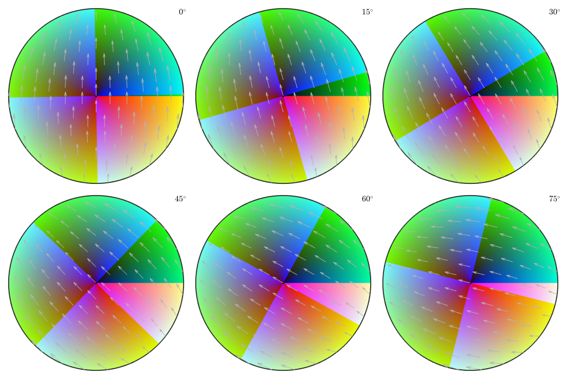
Lets visualize the orientation map by plotting it in orientation space as phi_2 sections
plot(oM,'sections',6,'phi2')

Although this visualization looks very smooth, the orientation map using Euler angles introduces lots of color jumps, i.e., the point 2 of our requirement list is not satisfied. This becomes obvious when plotting the colors as sigma sections, i.e., when section according to phi_1 - phi_2
plot(oM,'sections',6,'sigma')
Colorcoding according to inverse pole figure
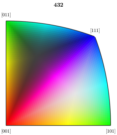
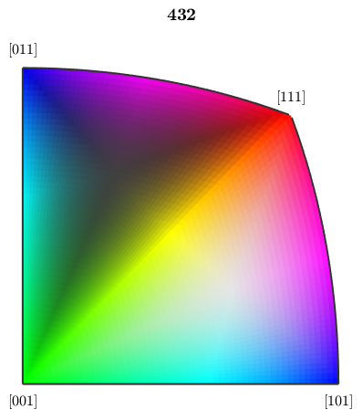
The standard way of mapping orientations to colors is based on inverse pole figures. The following orientation map assigns a color to each direction of the fundamental sector of the inverse pole figure
oM = ipfHSVKey(cs)

plot(oM)
oM =
  ipfHSVKey with properties:

             colorPostRotation: [1×1 rotation]
               colorStretching: 1
                   whiteCenter: [1×1 vector3d]
                     grayValue: [0.2000 0.5000]
                  grayGradient: 0.5000
                      maxAngle: Inf
    inversePoleFigureDirection: [1×1 vector3d]
                        dirMap: [1×1 HSVDirectionKey]
                           CS1: [6×4 crystalSymmetry]
                           CS2: [1×1 specimenSymmetry]
                     antipodal: 0
We may also look at the inverse pole figure sphere in 3d. One can nicely observe how the color map follows the given symmetry group.
close all
plot(oM,'3d')

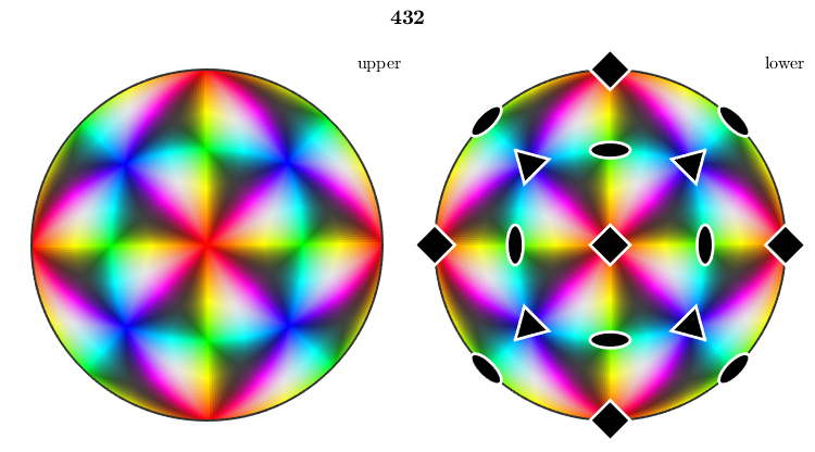
Alternatively, we may plot the color mapping in 2d on the entire sphere together with the symmetry elements
plot(oM,'complete')

hold on
plot(cs)
hold off
The orientation map provides several options to alter the alignment of the colors. Lets give some examples
% we may interchange green and blue by setting
oM.colorPostRotation = reflection(yvector);

plot(oM)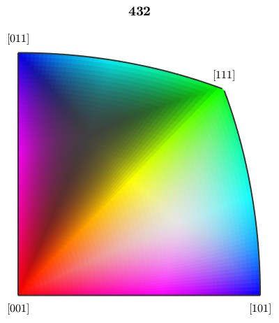
or shift the cycle of colors red, green, blue by
oM.colorPostRotation = rotation.byAxisAngle(zvector,120*degree);

plot(oM)
Lets now consider an EBSD map
mtexdata forsterite

plot(ebsd)
and assume we want to colorize the Forsterite phase according to its orientation. Then we first define the orientation mapping. Note that we can pass the phase we want to color instead of the crysta symmetry
oM = ipfHSVKey(ebsd('Forsterite'))oM =
ipfHSVKey with properties:
colorPostRotation: [1×1 rotation]
colorStretching: 1
whiteCenter: [1×1 vector3d]
grayValue: [0.2000 0.5000]
grayGradient: 0.5000
maxAngle: Inf
inversePoleFigureDirection: [1×1 vector3d]
dirMap: [1×1 HSVDirectionKey]
CS1: [4×2 crystalSymmetry]
CS2: [1×1 specimenSymmetry]
antipodal: 0
We may also want to set the inverse pole figure direction. This is done by
oM.inversePoleFigureDirection = zvector;
Next we compute the color corresponding to each orientation we want to plot.
color = oM.orientation2color(ebsd('Forsterite').orientations);Finally, we can use these colors to visualize the orientations of the Forsterite phase
plot(ebsd('Forsterite'),color)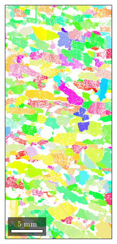
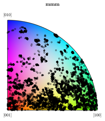
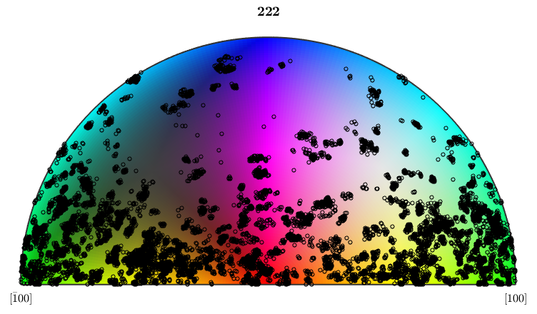
We can visualize the orientations of the forsterite phase also the other way round by plotting them into the inverse pole figure map.
plot(oM)

hold on
plotIPDF(ebsd('Forsterite').orientations,oM.inversePoleFigureDirection,...
  'MarkerSize',4,'MarkerFaceColor','none','MarkerEdgeColor','k')
hold off
I'm plotting 12500 random orientations out of 152345 given orientations
Since orientations measured by EBSD devices are pure rotations specified by its Euler angles, we may restrict the crystal symmetry group to pure rotations as well. As this group is smaller, in general, the corresponding fundamental sector is larger, which allows distinguishing more rotations
% this restricts the crystal symmetries used for visualization
% to proper rotations
ebsd('Forsterite').CS = ebsd('Forsterite').CS.properGroup;
oM = ipfHSVKey(ebsd('Forsterite'))

%
plot(oM)
oM =
  ipfHSVKey with properties:

             colorPostRotation: [1×1 rotation]
               colorStretching: 1
                   whiteCenter: [1×1 vector3d]
                     grayValue: [0.2000 0.5000]
                  grayGradient: 0.5000
                      maxAngle: Inf
    inversePoleFigureDirection: [1×1 vector3d]
                        dirMap: [1×1 HSVDirectionKey]
                           CS1: [4×1 crystalSymmetry]
                           CS2: [1×1 specimenSymmetry]
                     antipodal: 0
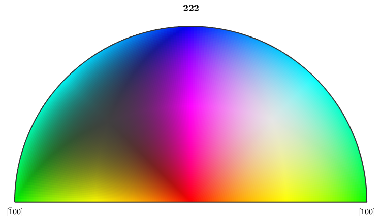
We observe that the fundamental sector is twice as large as for the original crystal symmetry. Furthermore, the measured Euler angles are not symmetric within this enlarged fundamental sector
hold on
plotIPDF(ebsd('Forsterite').orientations,oM.inversePoleFigureDirection,...
  'MarkerSize',4,'MarkerFaceColor','none','MarkerEdgeColor','k')
hold off
I'm plotting 25000 random orientations out of 152345 given orientations
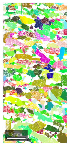
Lets finish this example by plotting the ebsd map of the Forsterite orientations color mapped according to this restricted symmetry group. The advantage of restricting the symmetry group is that we can distinguish more grains.
color = oM.orientation2color(ebsd('Forsterite').orientations);

plot(ebsd('Forsterite'),color)
| DocHelp 0.1 beta |