CSL Boundaries
Explains how to analyze CSL grain boundaries
Data import and grain detection
Lets import some iron data and segment grains within the data set.
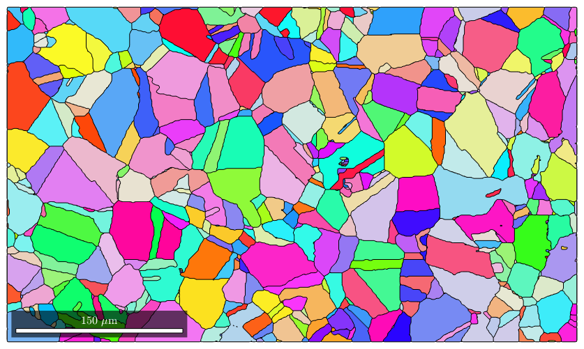
mtexdata csl
plotx2east

% grain segementation
[grains,ebsd.grainId] = calcGrains(ebsd('indexed'));

% grain smoothing
grains = smooth(grains,2);

% plot the result
plot(grains,grains.meanOrientation)
 loading data ...
 saving data to /home/hielscher/mtex/master/data/csl.mat
  I'm going to colorize the orientation data with the
  standard MTEX colorkey. To view the colorkey do:

  colorKey = ipfColorKey(ori_variable_name)
  plot(colorKey)
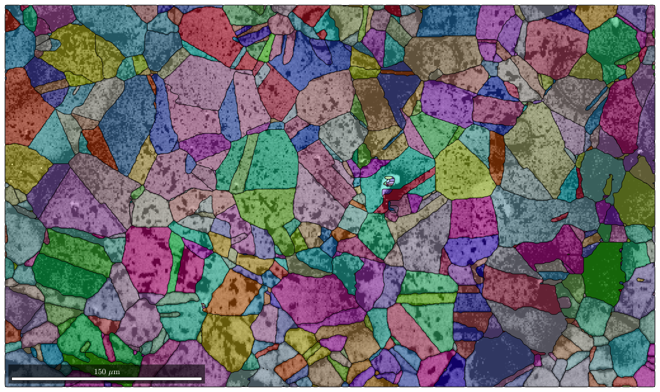
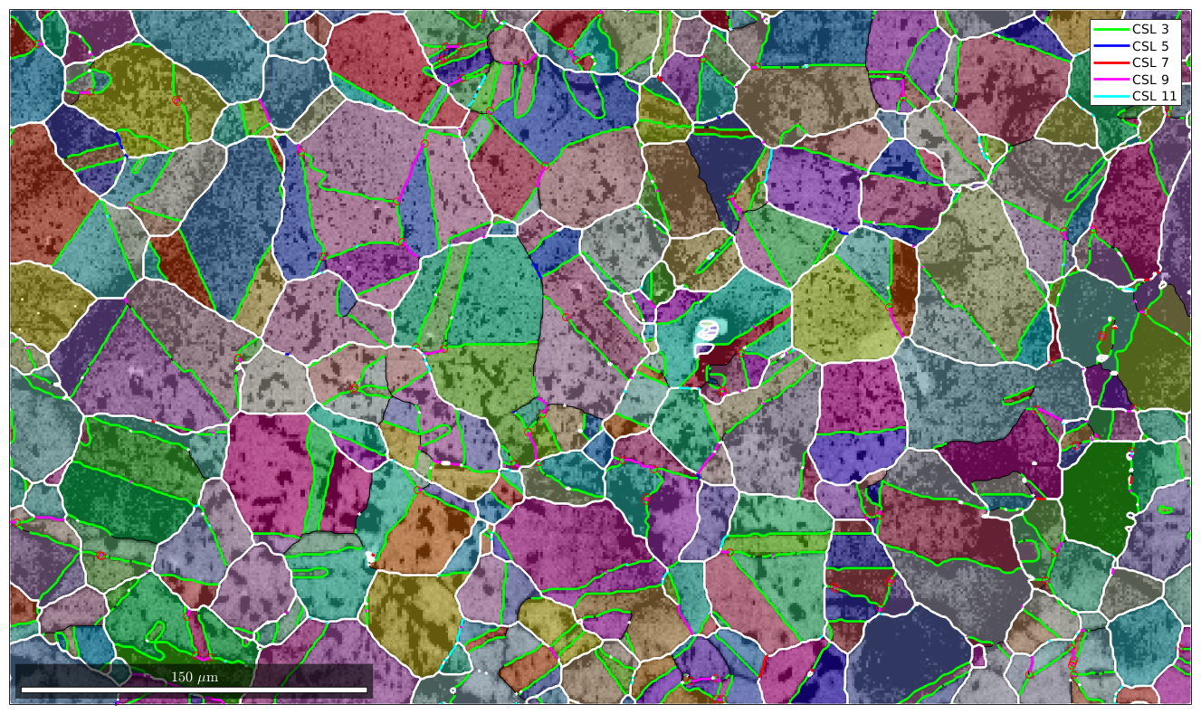
Next we plot image quality as it makes the grain boundaries visible. and overlay it with the orientation map
plot(ebsd,log(ebsd.prop.iq),'figSize','large')
mtexColorMap black2white
CLim(gcm,[.5,5])

% the option 'FaceAlpha',0.4 makes the plot a bit transluent
hold on
plot(grains,grains.meanOrientation,'FaceAlpha',0.4)
hold off
  I'm going to colorize the orientation data with the
  standard MTEX colorkey. To view the colorkey do:

  colorKey = ipfColorKey(ori_variable_name)
  plot(colorKey)
Detecting CSL Boundaries
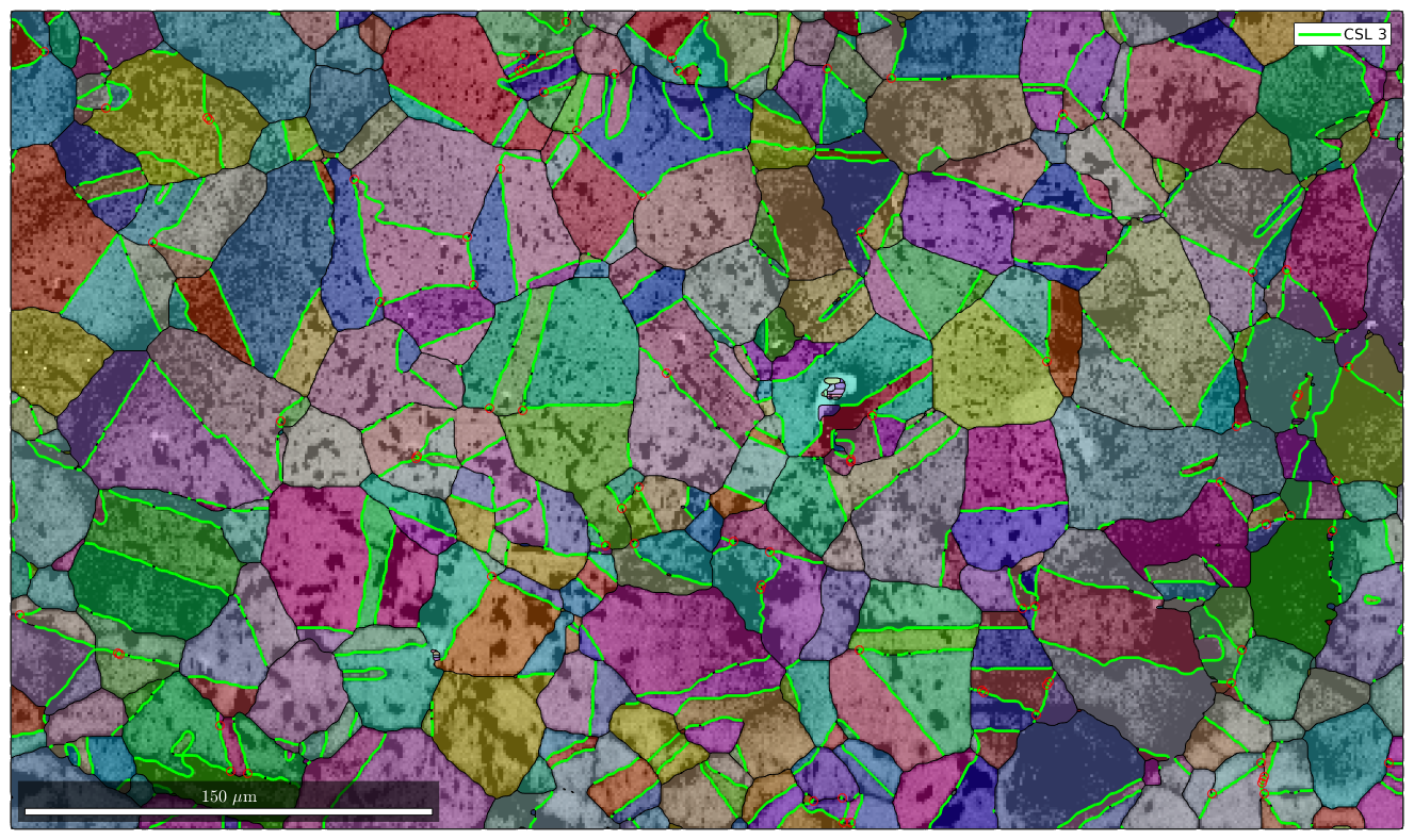
In order to detect CSL boundaries within the data set we first restrict the grain boundaries to iron to iron phase transitions and check then the boundary misorientations to be a CSL(3) misorientation with threshold of 3 degree.
% restrict to iron to iron phase transition
gB = grains.boundary('iron','iron')

% select CSL(3) grain boundaries
gB3 = gB(angle(gB.misorientation,CSL(3,ebsd.CS)) < 3*degree);

% overlay CSL(3) grain boundaries with the existing plot
hold on
plot(gB3,'lineColor','g','linewidth',2,'DisplayName','CSL 3')
hold off
gB = grainBoundary

 Segments  mineral 1  mineral 2
    20356       iron       iron

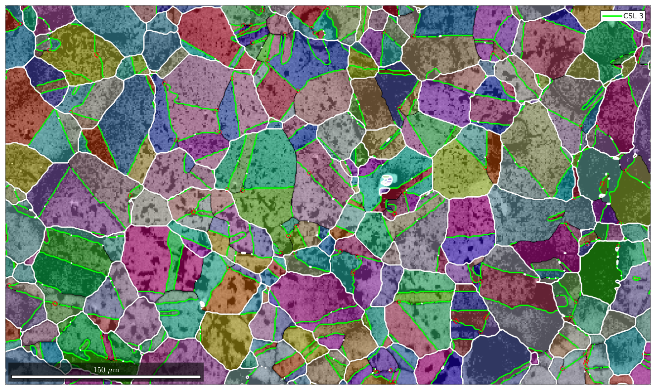
Mark triple points
Next we want to mark all triple points with at least 2 CSL boundaries
% logical list of CSL boundaries
isCSL3 = grains.boundary.isTwinning(CSL(3,ebsd.CS),3*degree);

% logical list of triple points with at least 2 CSL boundaries
tPid = sum(isCSL3(grains.triplePoints.boundaryId),2)>=2;

% plot these triple points
hold on
plot(grains.triplePoints(tPid),'color','r')
hold off
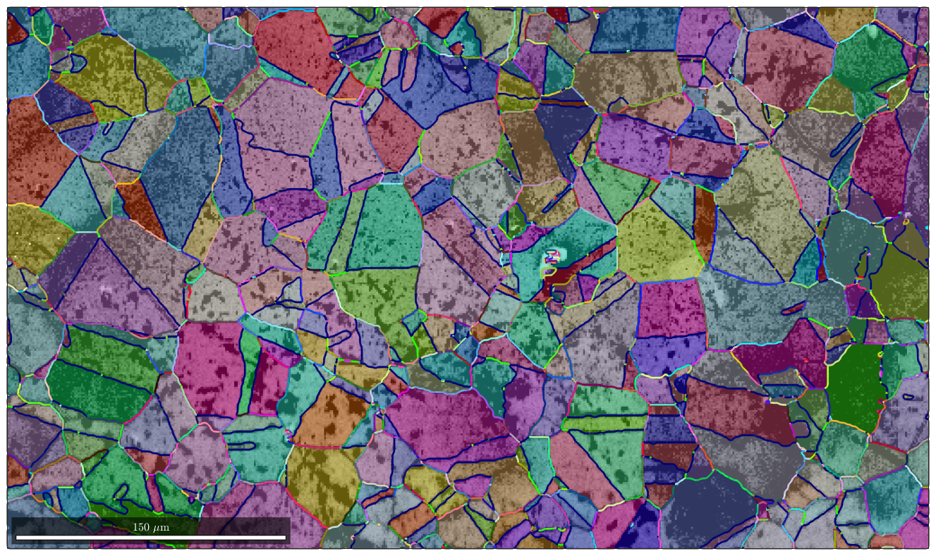
Merging grains with common CSL(3) boundary
Next we merge all grains together which have a common CSL(3) boundary. This is done with the command merge.
% this merges the grains
[mergedGrains,parentIds] = merge(grains,gB3);

% overlay the boundaries of the merged grains with the previous plot
hold on
plot(mergedGrains.boundary,'linecolor','w','linewidth',2)
hold off
Finaly, we check for all other types of CSL boundaries and overlay them with our plot.
delta = 5*degree;
gB5 = gB(gB.isTwinning(CSL(5,ebsd.CS),delta));
gB7 = gB(gB.isTwinning(CSL(7,ebsd.CS),delta));
gB9 = gB(gB.isTwinning(CSL(9,ebsd.CS),delta));
gB11 = gB(gB.isTwinning(CSL(11,ebsd.CS),delta));

hold on
plot(gB5,'lineColor','b','linewidth',2,'DisplayName','CSL 5')
hold on
plot(gB7,'lineColor','r','linewidth',2,'DisplayName','CSL 7')
hold on
plot(gB9,'lineColor','m','linewidth',2,'DisplayName','CSL 9')
hold on
plot(gB11,'lineColor','c','linewidth',2,'DisplayName','CSL 11')
hold off
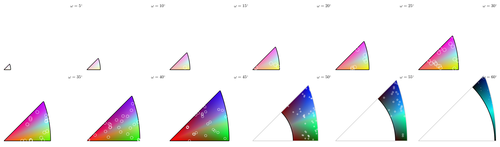
Colorizing misorientations
In the previous sections we have checked whether the boundary misorientations belong to certain specific classes of misorientations. In order to analyze the distribution of misorientations we may colorize the grain boundaries according to their misorientation. See S. Patala, J. K. Mason, and C. A. Schuh, 2012, for details. The coresponding orientation to color mapping is implemented into MTEX as
moriKey = PatalaColorKey(gB)
moriKey =
  PatalaColorKey with properties:

          CS1: [24×2 crystalSymmetry]
          CS2: [24×2 crystalSymmetry]
    antipodal: 1
Colorizing the grain boundaries is now straight forward
plot(ebsd,log(ebsd.prop.iq),'figSize','large')
mtexColorMap black2white
CLim(gcm,[.5,5])

% and overlay it with the orientation map
hold on
plot(grains,grains.meanOrientation,'FaceAlpha',0.4)

hold on
plot(gB,moriKey.orientation2color(gB.misorientation),'linewidth',2)
hold off
  I'm going to colorize the orientation data with the
  standard MTEX colorkey. To view the colorkey do:

  colorKey = ipfColorKey(ori_variable_name)
  plot(colorKey)
Lets examine the colormap. We plot it as axis angle sections and add 300 random boundary misorientations on top of it. Note that in this plot misorientations mori and inv(mori) are associated.
plot(moriKey,'axisAngle',(5:5:60)*degree)

plot(gB.misorientation,'points',300,'add2all',...
  'MarkerFaceColor','none','MarkerEdgeColor','w')
plotting 300 random orientations out of 20356 given orientations
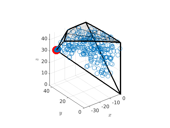
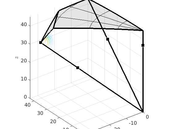
Misorientations in the 3d fundamental zone
We can also look at the boundary misorienations in the 3 dimensional fundamental orientation zone.
% compute the boundary of the fundamental zone
oR = fundamentalRegion(moriKey.CS1,moriKey.CS2,'antipodal');
close all
plot(oR)

% plot 500 random misorientations in the 3d fundamenal zone
mori = discreteSample(gB.misorientation,500);
hold on
plot(mori.project2FundamentalRegion)
hold off


% mark the CSL(3) misorientation
hold on
csl3 = CSL(3,ebsd.CS);
plot(csl3.project2FundamentalRegion('antipodal') ,'MarkerColor','r','DisplayName','CSL 3','MarkerSize',20)
hold off
Analyzing the misorientation distribution function
In order to analyze more quantitatively the boundary misorientation distribution we can compute the so called misorientation distribution function. The option antipodal is applied since we want to identify mori and inv(mori).
mdf = calcMDF(gB.misorientation,'halfwidth',2.5*degree,'bandwidth',32)
mdf = MDF
  crystal symmetry : iron (m-3m)
  crystal symmetry : iron (m-3m)
  antipodal:         true

  Harmonic portion:
    degree: 32
    weight: 1
Next we can visualize the misorientation distribution function in axis angle sections.
plot(mdf,'axisAngle',(25:5:60)*degree,'colorRange',[0 15])

annotate(CSL(3,ebsd.CS),'label','$CSL_3$','backgroundcolor','w')
annotate(CSL(5,ebsd.CS),'label','$CSL_5$','backgroundcolor','w')
annotate(CSL(7,ebsd.CS),'label','$CSL_7$','backgroundcolor','w')
annotate(CSL(9,ebsd.CS),'label','$CSL_9$','backgroundcolor','w')

drawNow(gcm)
The MDF can be now used to compute prefered misorientations
mori = mdf.calcModes(2)
mori = misorientation
  size: 1 x 2
  crystal symmetry : iron (m-3m)
  crystal symmetry : iron (m-3m)

  Bunge Euler angles in degree
     phi1     Phi    phi2    Inv.
   243.71 48.3206 152.606       0
  98.0317 38.0679 227.755       0
and their volumes in percent
100 * volume(gB.misorientation,CSL(3,ebsd.CS),2*degree)

100 * volume(gB.misorientation,CSL(9,ebsd.CS),2*degree)
ans =
   40.9904
ans =
    2.0338
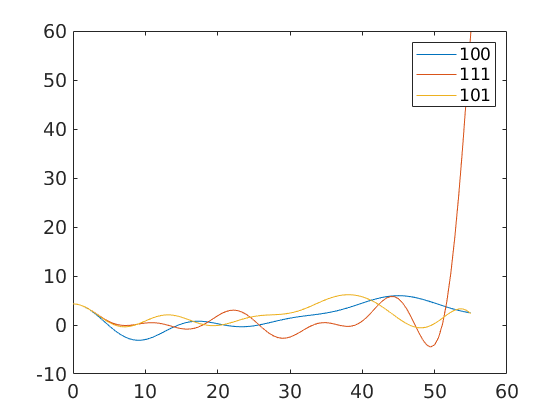
or to plot the MDF along certain fibres
omega = linspace(0,55*degree);
fibre100 = orientation.byAxisAngle(xvector,omega,mdf.CS,mdf.SS)
fibre111 = orientation.byAxisAngle(vector3d(1,1,1),omega,mdf.CS,mdf.SS)
fibre101 = orientation.byAxisAngle(vector3d(1,0,1),omega,mdf.CS,mdf.SS)

close all
plot(omega ./ degree,mdf.eval(fibre100))
hold on
plot(omega ./ degree,mdf.eval(fibre111))
plot(omega ./ degree,mdf.eval(fibre101))
hold off
legend('100','111','101')
fibre100 = misorientation
  size: 1 x 100
  crystal symmetry : iron (m-3m)
  crystal symmetry : iron (m-3m)


fibre111 = misorientation
  size: 1 x 100
  crystal symmetry : iron (m-3m)
  crystal symmetry : iron (m-3m)


fibre101 = misorientation
  size: 1 x 100
  crystal symmetry : iron (m-3m)
  crystal symmetry : iron (m-3m)
or to evaluate it in an misorientation directly
mori = orientation.byEuler(15*degree,28*degree,14*degree,mdf.CS,mdf.CS)

mdf.eval(mori)
mori = misorientation
  size: 1 x 1
  crystal symmetry : iron (m-3m)
  crystal symmetry : iron (m-3m)

  Bunge Euler angles in degree
  phi1  Phi phi2 Inv.
    15   28   14    0

ans =
    5.6826
| DocHelp 0.1 beta |