Grain Boundaries
Overview about colorizing grain boundaries
| On this page ... |
| The grain boundary |
| Visualizing special grain boundaries |
| Phase boundaries |
| Subboundaries |
| Misorientation |
| Classifying special boundaries |
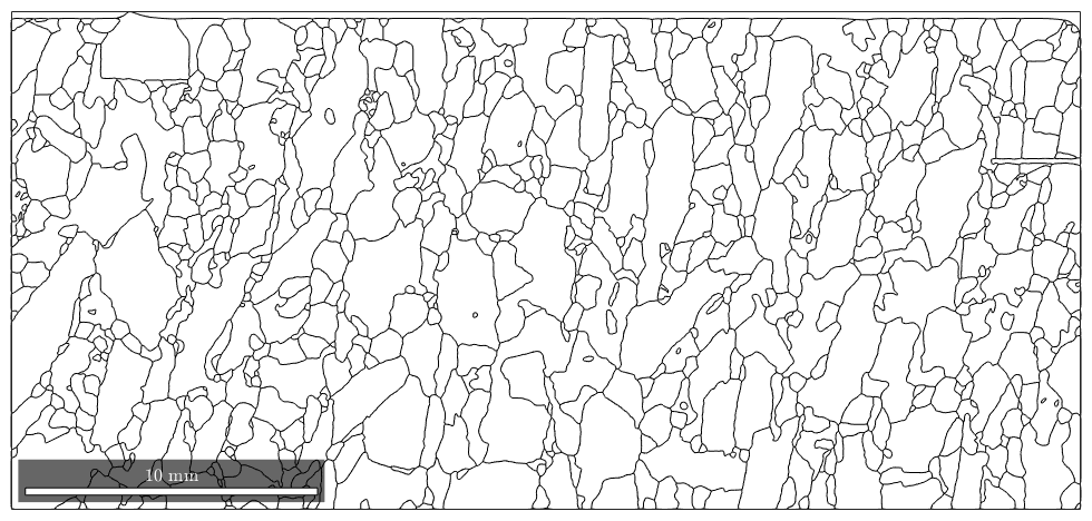
Let's import some EBSD data and compute the grains.
close all
mtexdata forsterite
plotx2east

ebsd = ebsd('indexed');
[grains,ebsd.grainId] = calcGrains(ebsd);

% remove very small grains
ebsd(grains(grains.grainSize<=5)) = [];

% and recompute grains
[grains,ebsd.grainId] = calcGrains(ebsd);

% smooth the grains a bit
grains =smooth(grains,4)
grains = grain2d

 Phase  Grains  Pixels     Mineral  Symmetry  Crystal reference frame
     1     426  151466  Forsterite       mmm
     2     200   25635   Enstatite       mmm
     3     142    7306    Diopside     12/m1       X||a*, Y||b*, Z||c

 boundary segments: 33636
 triple points: 1347

 Properties: GOS, meanRotation
The grain boundary
The grain boundary of a list of grains can be extracted by
gB = grains.boundary

plot(gB)
gB = grainBoundary

 Segments   mineral 1   mineral 2
     1355  notIndexed  Forsterite
      198  notIndexed   Enstatite
       36  notIndexed    Diopside
    13890  Forsterite  Forsterite
    10857  Forsterite   Enstatite
     5167  Forsterite    Diopside
      598   Enstatite   Enstatite
     1259   Enstatite    Diopside
      276    Diopside    Diopside
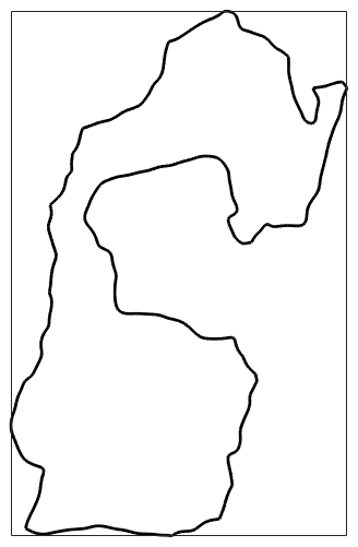
Accordingly, we can access the grain boundary of a specific grain by
grains(267).boundary

plot(grains(267).boundary,'lineWidth',2,'micronbar','off')
ans = grainBoundary

 Segments   mineral 1   mineral 2
      304  Forsterite  Forsterite
      126  Forsterite   Enstatite
       97  Forsterite    Diopside
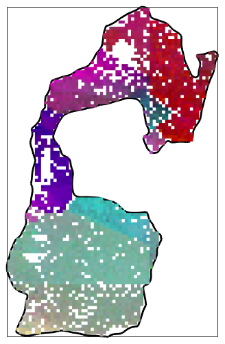
Let's combine it with the orientation measurements inside select axisAngle color key. This colorizes the mean orientation gray and deviations from the mean orientation according to the misorientation axis where saturation increases with the misorientation angle
ipfKey = axisAngleColorKey(grains(267));

% set the reference orientation to be the grain mean orientation
ipfKey.oriRef = grains(267).meanOrientation;
ipfKey.maxAngle = 4*degree;

% get the ebsd data of grain 267
ebsd_267 = ebsd(grains(267));

% plot the orientation data
hold on
plot(ebsd_267,ipfKey.orientation2color(ebsd_267.orientations))
hold off
Visualizing special grain boundaries
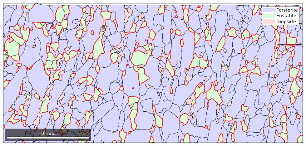
Phase boundaries
For a multi-phase system, the location of specific phase transistions may be of interest. The following plot highlights all Forsterite to Enstatite phase transitions
close all
plot(grains,'faceAlpha',.3)
hold on
plot(grains.boundary('Fo','En'),'linecolor','r','linewidth',1.5)
hold off
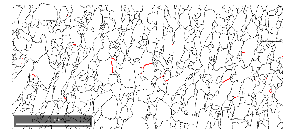
Subboundaries
Another type of boundaries is boundaries between measurements that belong to the same grain. This happens if a grain has a texture gradient that loops around these two measurements.
close all
plot(grains.boundary)
hold on
plot(grains.innerBoundary,'linecolor','r','linewidth',2)
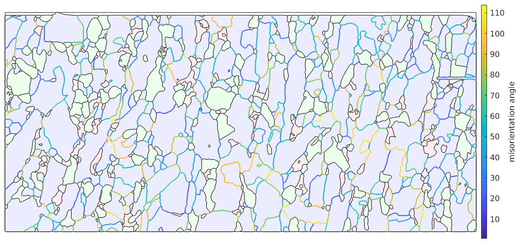
Misorientation
The boundary misorientation is the misorientation between the two neighboring pixels of a boundary segment. Depending of the misorientation angle one distinguishes between high angle and low angle grain boundaries. In MTEX we can visualize the boundary misorientation angle by the commands
close all
gB_Fo = grains.boundary('Fo','Fo');
plot(grains,'translucent',.3,'micronbar','off')
legend off
hold on
plot(gB_Fo,gB_Fo.misorientation.angle./degree,'linewidth',1.5)
hold off
mtexColorbar('title','misorientation angle')
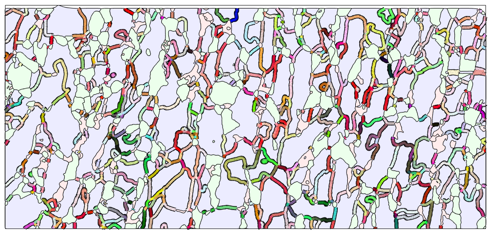
In order to visuale the full misorientation, i.e., axis and angle, one has to define a corresponding color key. One option is the color key described in the paper by S. Patala, J. K. Mason, and C. A. Schuh, Improved representations of misorientation information for grain boundary, Prog. Mater. Sci., vol. 57, no. 8, pp. 1383-1425, 2012.
close all
plot(grains,'translucent',.3,'micronbar','off')
legend off
hold on

% this reorders the boundary segement a a connected graph which results in
% a smoother plot
gB_Fo = gB_Fo.reorder;

ipfKey = PatalaColorKey(gB_Fo);

plot(gB_Fo,'linewidth',6)
% on my computer setting the renderer to painters gives a much more
% pleasent result
%set(gcf,'Renderer','painters')
hold on

plot(gB_Fo,ipfKey.orientation2color(gB_Fo.misorientation),'linewidth',4)

hold off
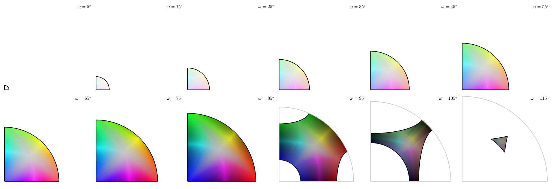
Lets visualize the color key as axis angle sections through the misorientation space
plot(ipfKey)
Classifying special boundaries
Actually, it might be more informative, if we classify the grain boundaries after some special property.
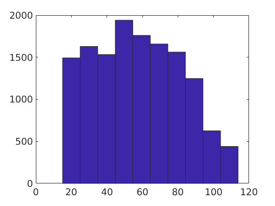
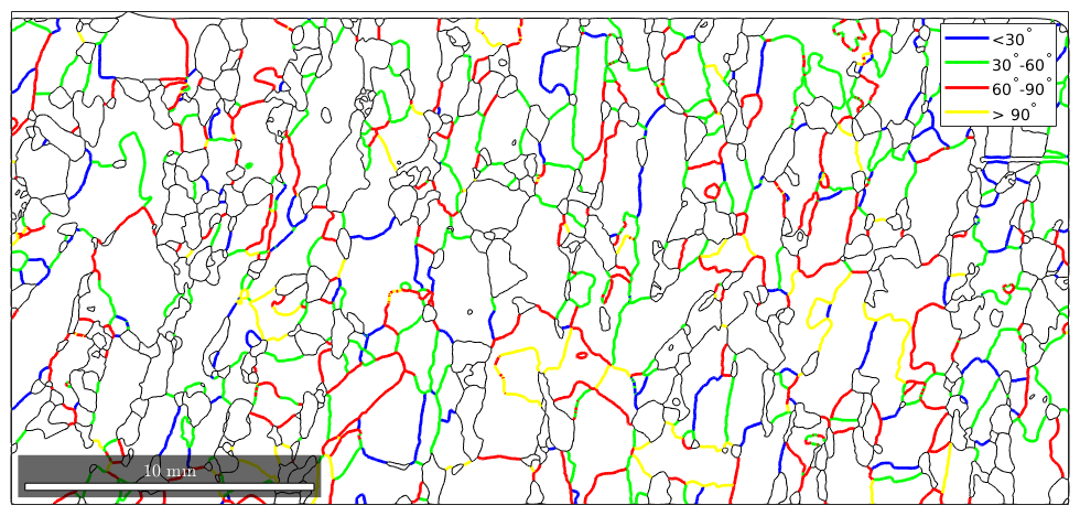
We can mark grain boundaries after its misorientation angle is in a certain range
close all

mAngle = gB_Fo.misorientation.angle./ degree;
hist(mAngle) [~,id] = histc(mAngle,0:30:120);
plot(gB,'linecolor','k')

hold on
plot(gB_Fo(id==1),'linecolor','b','linewidth',2,'DisplayName','<30^\circ')
plot(gB_Fo(id==2),'linecolor','g','linewidth',2,'DisplayName','30^\circ-60^\circ')
plot(gB_Fo(id==3),'linecolor','r','linewidth',2,'DisplayName','60^\circ-90^\circ')
plot(gB_Fo(id==4),'linecolor','y','linewidth',2,'DisplayName','> 90^\circ')

hold off
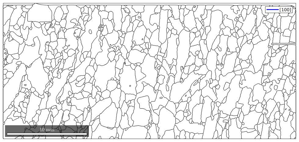
Or we mark the rotation axis of the misorientation.
close all
plot(gB)
hold on

ind = angle(gB_Fo.misorientation.axis,xvector)<5*degree;

plot(gB_Fo(ind),'linecolor','b','linewidth',2,'DisplayName','[100]')
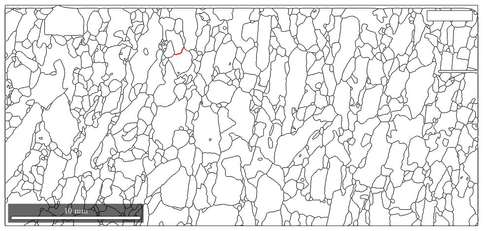
Or we mark a special rotation between neighboured grains. If a linecolor is not specified, then the boundary is colorcoded after its angular difference to the given rotation.
rot = rotation.byAxisAngle(vector3d(1,1,1),60*degree);
ind = angle(gB_Fo.misorientation,rot)<10*degree;

close all
plot(gB)
hold on
plot(gB_Fo(ind),'lineWidth',1.5,'lineColor','r')

legend('>2^\circ','60^\circ/[001]')
Warning: Ignoring extra legend entries.
Another kind of special boundaries is tilt and twist boundaries. We can find a tilt boundary by specifying the crystal form,
which is tilted, i.e. the misorientation maps a lattice plane  of on grain onto the others grain lattice plane.
where  are neighbored orientations. TODO
%close all
%plot(grains.boundary)
%hold on
%plot(grains.boundary,'property',Miller(1,1,1),'delta',2*degree,...
%  'linecolor','r','linewidth',1.5)
%plot(grains.boundary,'property',Miller(0,0,1),'delta',2*degree,...
%  'linecolor','b','linewidth',1.5)
%
%legend('>2^\circ',...
%  '\{111\}',...
%  '\{001\}')
| DocHelp 0.1 beta |