Misorientations at grain boundaries
Analyse misorientations along grain boundaries
This example explains how to analyse boundary misorientation by means of misorientation axes
Import EBSD data and select a subregion
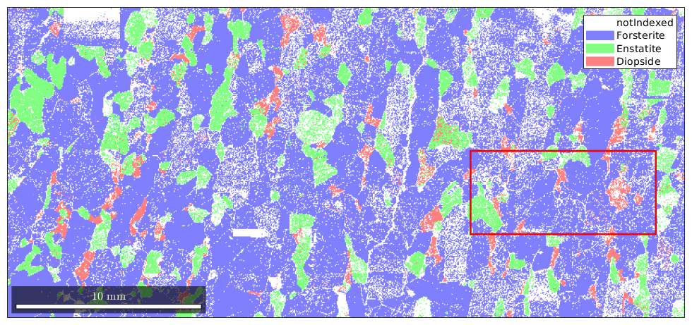
First step is as always to import the data. Here we restrict the big data set to a subregion to make the results easier to visulize
% take some MTEX data set
mtexdata forsterite
plotx2east

% define a sub region
xmin = 25000;
xmax = 35000;
ymin = 4500;
ymax = 9000;

region = [xmin ymin xmax-xmin ymax-ymin];

% visualize the whole data set
plot(ebsd)
% and marke the sub region
rectangle('position',region,'edgecolor','r','linewidth',2)

% select EBSD data within region
condition = inpolygon(ebsd,region); % select indices by polygon
ebsd = ebsd(condition);
Grain modelling
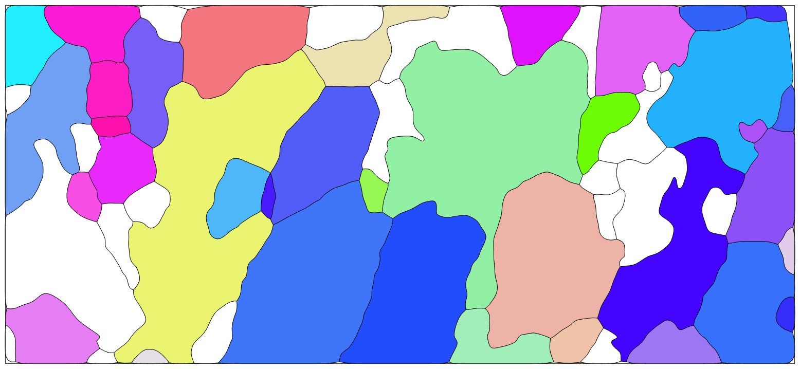
Second step is the modelling of the grains and grain boundaries
% segmentation angle typically 10 to 15 degrees that seperates to grains
seg_angle = 10;

% minimum indexed points per grain between 5 and 10
min_points = 10;

% restrict to indexed only points
[grains,ebsd.grainId,ebsd.mis2mean] = calcGrains(ebsd('indexed'),'angle',seg_angle*degree);

% remove small grains with less than min_points indexed points
grains = grains(grains.grainSize > min_points);

% re-calculate grain model to cleanup grain boundaries with less than
% minimum index points used ebsd points within grains having the minium
% indexed number of points (e.g. 10 points)
ebsd = ebsd(grains);
[grains,ebsd.grainId,ebsd.mis2mean] = calcGrains(ebsd('indexed'),'angle',seg_angle*degree);

% smooth grains
grains = smooth(grains,4);

% plot the data
% Note, only the forsterite grains are colorred. Grains with different
% phase remain white
plot(grains('fo'),grains('fo').meanOrientation,'micronbar','off','figSize','large')
hold on
plot(grains.boundary)
hold off
  I'm going to colorize the orientation data with the
  standard MTEX colorkey. To view the colorkey do:

  colorKey = ipfColorKey(ori_variable_name)
  plot(colorKey)
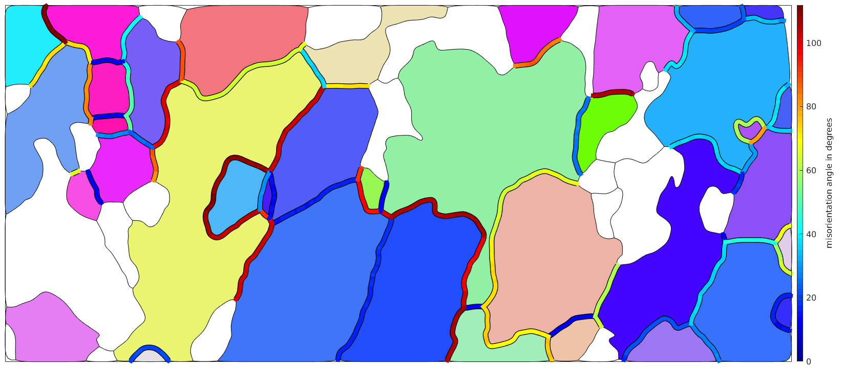
Visualize the misorientation angle at grain boundaries
% define the linewidth
lw = 6;

% consider on Fo-Fo boundaries
gB = grains.boundary('Fo','Fo');

% The following command reorders the boundary segments such that they are
% connected. This has two advantages:
% 1. the plots become more smooth
% 2. you can consider every third line segment as we do in the next paragraph
gB = gB.reorder;

% visualize the misorientation angle
% draw the boundary in black very thick
hold on
plot(gB,'linewidth',lw+2);

% and on top of it the boundary colorized according to the misorientation
% angle
hold on
plot(gB,gB.misorientation.angle./degree,'linewidth',lw);
hold off
mtexColorMap jet
mtexColorbar('title','misorientation angle in degrees')
Visualize the misorientation axes in specimen coordinates
Computing the misorientation axes in specimen coordinates can not be done using the boundary misorientations only. In fact, we require the orientations on both sides of the grain boundary. Lets extract them first.
% do only consider every third boundary segment
Sampling_N=3;
gB = gB(1:Sampling_N:end);

% the following command gives an Nx2 matrix of orientations which contains
% for each boundary segment the orientation on both sides of the boundary.
ori = ebsd(gB.ebsdId).orientations;

% the misorientation axis in specimen coordinates
gB_axes = axis(ori(:,1),ori(:,2));

% axes can be plotted using the command quiver
hold on
quiver(gB,gB_axes,'linewidth',1,'color','k','autoScaleFactor',0.3)
hold off
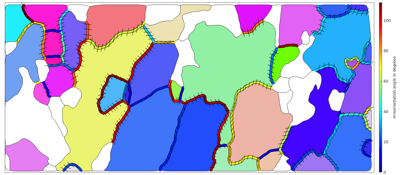
Note, the shorter the axes the more they stick out of the surface. What may be a bit surprising is that the misorientations axes have some abrupt changes at the left hands side grain boundary. The reason for this is that the misorientations angle at this boundary is close to the maximum misorientation angle of 120 degree. As a consequence, slight changes in the misorientation may leed to a completely different disorientation, i.e., a different but symmetrically equivalent misorientation has a smaller misorientation angle.
| DocHelp 0.1 beta |