
%{

 .sum files are generated by the program PF program
 https://www.ncnr.nist.gov/instruments/bt8/BT8DataAnalysis.htm


Written by Adam Creuziger (adam.creuziger@nist.gov)

Oct 2017

This data was developed by employees of the National Institute of Standards and Technology (NIST), an agency of the Federal Government. Pursuant to title 17 United States Code Section 105, works of NIST employees are not subject to copyright protection in the United States and are considered to be in the public domain.

The data is provided by NIST as a public service and is expressly provided "AS IS." NIST MAKES NO WARRANTY OF ANY KIND, EXPRESS, IMPLIED OR STATUTORY, INCLUDING, WITHOUT LIMITATION, THE IMPLIED WARRANTY OF MERCHANTABILITY, FITNESS FOR A PARTICULAR PURPOSE, NON-INFRINGEMENT AND DATA ACCURACY. NIST does not warrant or make any representations regarding the use of the data or the results thereof, including but not limited to the correctness, accuracy, reliability or usefulness of the data. NIST SHALL NOT BE LIABLE AND YOU HEREBY RELEASE NIST FROM LIABILITY FOR ANY INDIRECT, CONSEQUENTIAL, SPECIAL, OR INCIDENTAL DAMAGES (INCLUDING DAMAGES FOR LOSS OF BUSINESS PROFITS, BUSINESS INTERRUPTION, LOSS OF BUSINESS INFORMATION, AND THE LIKE), WHETHER ARISING IN TORT, CONTRACT, OR OTHERWISE, ARISING FROM OR RELATING TO THE DATA (OR THE USE OF OR INABILITY TO USE THIS DATA), EVEN IF NIST HAS BEEN ADVISED OF THE POSSIBILITY OF SUCH DAMAGES.

To the extent that NIST may hold copyright in countries other than the United States, you are hereby granted the non-exclusive irrevocable and unconditional right to print, publish, prepare derivative works and distribute the NIST data, in any medium, or authorize others to do so on your behalf, on a royalty-free basis throughout the world.

You may improve, modify, and create derivative works of the data or any portion of the data, and you may copy and distribute such modifications or works. Modified works should carry a notice stating that you changed the data and should note the date and nature of any such change. Please explicitly acknowledge the National Institute of Standards and Technology as the source of the data: Data citation recommendations are provided below.

Permission to use this data is contingent upon your acceptance of the terms of this agreement and upon your providing appropriate acknowledgments of NIST's creation of the data.

See: https://www.nist.gov/director/licensing
%}
Set preferences
%clear the workspace and close open windows
clc
clear
close all

% set to 1 to remove extra annotations
setMTEXpref('FontSize',1);

% To align pole figures with mplstereonet,
plotx2north % X up, Y to the left

% all paths below are built from here, so the script no longer depends on
% the current directory being JACCreuziger
jacPath = fullfile(mtexExamplePath,'JACCreuziger');

%color map
run(fullfile(jacPath,'ColorMap4.m'))

% Only read in TRIP 700 pole figures to plot
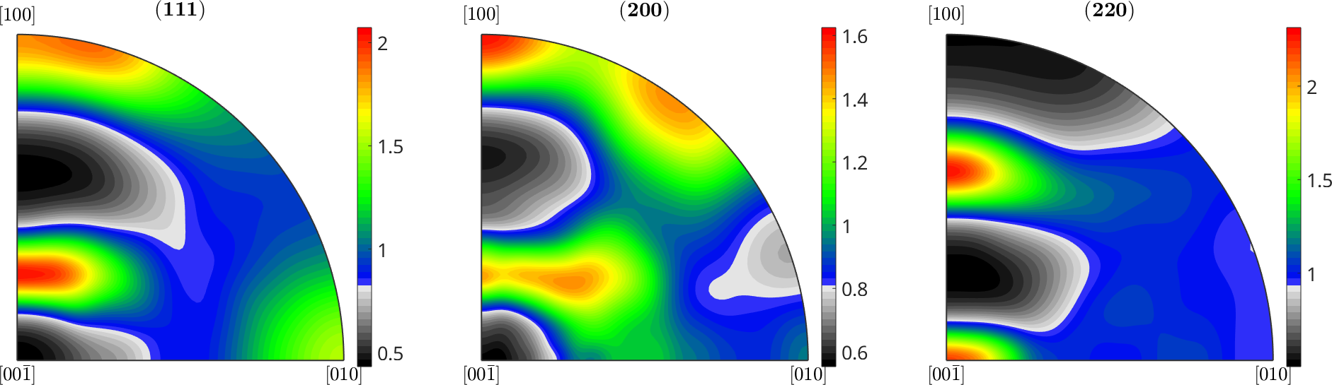
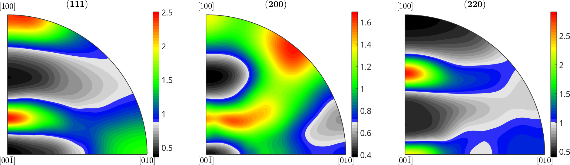
% austenite - 111, 200, 220
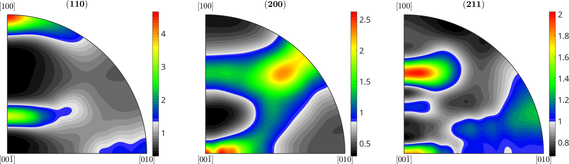
% ferrite - 110, 200, 211

% plot as quarter circles
Set sample and crystal symmetry
cs = crystalSymmetry('m-3m');
ss = specimenSymmetry('orthorhombic');


%austenite and ferrite pole figures to plot
h_ferrite = {Miller(1,1,0,cs),Miller(2,0,0,cs),Miller(2,1,1,cs)} ;
h_austenite = {Miller(1,1,1,cs),Miller(2,0,0,cs),Miller(2,2,0,cs)} ;

%SavePaths
savepath=fullfile(jacPath,'ExpFigures');
mkdir(savepath)


%Create a file with the sample name, texture intex and texture entropy
fileID = fopen(strcat(savepath,'/','ExpTextureValues.txt'),'w');

fprintf(fileID,'%12s\t %5s\t %5s\n','Name','TI', 'Ent');
fclose(fileID);
Warning: Directory already exists.read in 4 experimental data sets
Each pole figure is rebuilt with its crystal direction stated explicitly. loadPoleFigure_generic otherwise guesses the Miller index from the file name, which reads the 426 of '110F-Creuz426sym.sum' as a second crystal direction and leaves a pole figure that calcODF cannot invert.
for i=1:4if i==1
disp('TRIP 700 Ferrite')
bname='TRIP700F';
phase ='ferrite';
pname = [fullfile(jacPath,'ExperimentalData','TRIP700') filesep];
pf1T=loadPoleFigure_generic([pname '110F-d4.sum'], 'HEADER',1,'degree','ColumnNames',{'polar angle','azimuth angle','intensity'},'Columns',[2 1 3]);
pf1B=loadPoleFigure_generic([pname '110F-d4.sum'], 'HEADER',1,'degree','ColumnNames',{'polar angle','azimuth angle','intensity'},'Columns',[2 1 4]);
pf1 = correct(pf1T,'background',pf1B);
pf1 = PoleFigure(Miller(1,1,0,cs),pf1.r,pf1.intensities,cs,ss);
pf2T=loadPoleFigure_generic([pname '200F-d4.sum'], 'HEADER',1,'degree','ColumnNames',{'polar angle','azimuth angle','intensity'},'Columns',[2 1 3]);
pf2B=loadPoleFigure_generic([pname '200F-d4.sum'], 'HEADER',1,'degree','ColumnNames',{'polar angle','azimuth angle','intensity'},'Columns',[2 1 4]);
pf2 = correct(pf2T,'background',pf2B);
pf2 = PoleFigure(Miller(2,0,0,cs),pf2.r,pf2.intensities,cs,ss);
pf3T=loadPoleFigure_generic([pname '211F-d4.sum'], 'HEADER',1,'degree','ColumnNames',{'polar angle','azimuth angle','intensity'},'Columns',[2 1 3]);
pf3B=loadPoleFigure_generic([pname '211F-d4.sum'], 'HEADER',1,'degree','ColumnNames',{'polar angle','azimuth angle','intensity'},'Columns',[2 1 4]);
pf3 = correct(pf3T,'background',pf3B);
pf3 = PoleFigure(Miller(2,1,1,cs),pf3.r,pf3.intensities,cs,ss);
pfF=[pf1,pf2,pf3];
%figure; plot(pfF); colorbar;
odf = calcODF(pfF, cs,ss, 'halfwidth',5*degree, 'resolution',5*degree);
%figure; plot(odf,'phi2','sections',18,'projection','plain','minmax', 'off',cs,ss);setColorRange(gcm,[0, 4]);mtexColorbar;
elseif i==2
%TRIP 700 Austenite
disp('TRIP 700 Austenite')
bname='TRIP700A';
phase ='austenite';
pname = [fullfile(jacPath,'ExperimentalData','TRIP700') filesep];
pf1T=loadPoleFigure_generic([pname '200A-d4.sum'], 'HEADER',1,'degree','ColumnNames',{'polar angle','azimuth angle','intensity'},'Columns',[2 1 3]);
pf1B=loadPoleFigure_generic([pname '200A-d4.sum'], 'HEADER',1,'degree','ColumnNames',{'polar angle','azimuth angle','intensity'},'Columns',[2 1 4]);
pf1 = correct(pf1T,'background',pf1B);
pf1 = PoleFigure(Miller(2,0,0,cs),pf1.r,pf1.intensities,cs,ss);
pf2T=loadPoleFigure_generic([pname '220A-d4.sum'], 'HEADER',1,'degree','ColumnNames',{'polar angle','azimuth angle','intensity'},'Columns',[2 1 3]);
pf2B=loadPoleFigure_generic([pname '220A-d4.sum'], 'HEADER',1,'degree','ColumnNames',{'polar angle','azimuth angle','intensity'},'Columns',[2 1 4]);
pf2 = correct(pf2T,'background',pf2B);
pf2 = PoleFigure(Miller(2,2,0,cs),pf2.r,pf2.intensities,cs,ss);
pf3T=loadPoleFigure_generic([pname '311A-d4.sum'], 'HEADER',1,'degree','ColumnNames',{'polar angle','azimuth angle','intensity'},'Columns',[2 1 3]);
pf3B=loadPoleFigure_generic([pname '311A-d4.sum'], 'HEADER',1,'degree','ColumnNames',{'polar angle','azimuth angle','intensity'},'Columns',[2 1 4]);
pf3 = correct(pf3T,'background',pf3B);
pf3 = PoleFigure(Miller(3,1,1,cs),pf3.r,pf3.intensities,cs,ss);
pfF=[pf1,pf2,pf3];
%figure; plot(pfF); colorbar;
odf = calcODF(pfF, cs,ss, 'halfwidth',5*degree, 'resolution',5*degree);
elseif i==3
%TRIP 780 Austenite
disp('TRIP 780 Austenite')
bname='TRIP780A';
phase ='austenite';
pname = [fullfile(jacPath,'ExperimentalData','TRIP780') filesep];
pf1T=loadPoleFigure_generic([pname '200A-Creuz427sym.sum'], 'HEADER',1,'degree','ColumnNames',{'polar angle','azimuth angle','intensity'},'Columns',[2 1 3]);
pf1B=loadPoleFigure_generic([pname '200A-Creuz427sym.sum'], 'HEADER',1,'degree','ColumnNames',{'polar angle','azimuth angle','intensity'},'Columns',[2 1 4]);
pf1 = correct(pf1T,'background',pf1B);
pf1 = PoleFigure(Miller(2,0,0,cs),pf1.r,pf1.intensities,cs,ss);
pf2T=loadPoleFigure_generic([pname '220A-Creuz429sym.sum'], 'HEADER',1,'degree','ColumnNames',{'polar angle','azimuth angle','intensity'},'Columns',[2 1 3]);
pf2B=loadPoleFigure_generic([pname '220A-Creuz429sym.sum'], 'HEADER',1,'degree','ColumnNames',{'polar angle','azimuth angle','intensity'},'Columns',[2 1 4]);
pf2 = correct(pf2T,'background',pf2B);
pf2 = PoleFigure(Miller(2,2,0,cs),pf2.r,pf2.intensities,cs,ss);
pfF=[pf1,pf2];
%figure; plot(pfF); colorbar;
odf = calcODF(pfF, cs,ss, 'halfwidth',5*degree, 'resolution',5*degree);
elseif i==4
%TRIP 780 Ferrite
disp('TRIP 780 Ferrite')
bname='TRIP780F';
phase ='ferrite';
pname = [fullfile(jacPath,'ExperimentalData','TRIP780') filesep];
pf1T=loadPoleFigure_generic([pname '110F-Creuz426sym.sum'], 'HEADER',1,'degree','ColumnNames',{'polar angle','azimuth angle','intensity'},'Columns',[2 1 3]);
pf1B=loadPoleFigure_generic([pname '110F-Creuz426sym.sum'], 'HEADER',1,'degree','ColumnNames',{'polar angle','azimuth angle','intensity'},'Columns',[2 1 4]);
pf1 = correct(pf1T,'background',pf1B);
pf1 = PoleFigure(Miller(1,1,0,cs),pf1.r,pf1.intensities,cs,ss);
pf2T=loadPoleFigure_generic([pname '200F-Creuz428sym.sum'], 'HEADER',1,'degree','ColumnNames',{'polar angle','azimuth angle','intensity'},'Columns',[2 1 3]);
pf2B=loadPoleFigure_generic([pname '200F-Creuz428sym.sum'], 'HEADER',1,'degree','ColumnNames',{'polar angle','azimuth angle','intensity'},'Columns',[2 1 4]);
pf2 = correct(pf2T,'background',pf2B);
pf2 = PoleFigure(Miller(2,0,0,cs),pf2.r,pf2.intensities,cs,ss);
pf3T=loadPoleFigure_generic([pname '211F-Creuz431sym.sum'], 'HEADER',1,'degree','ColumnNames',{'polar angle','azimuth angle','intensity'},'Columns',[2 1 3]);
pf3B=loadPoleFigure_generic([pname '211F-Creuz431sym.sum'], 'HEADER',1,'degree','ColumnNames',{'polar angle','azimuth angle','intensity'},'Columns',[2 1 4]);
pf3 = correct(pf3T,'background',pf3B);
pf3 = PoleFigure(Miller(2,1,1,cs),pf3.r,pf3.intensities,cs,ss);
pfF=[pf1,pf2,pf3];
%figure; plot(pfF); colorbar;
odf = calcODF(pfF, cs,ss, 'halfwidth',5*degree, 'resolution',5*degree);
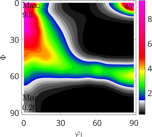
endTRIP 700 FerriteTRIP 700 AusteniteTRIP 780 AusteniteTRIP 780 FerriteCreate Plots
disp('Create Plots')


if strcmp(bname,'TRIP780F')
    % use a different colormap for expanded range of ODF
    % This colormap range overlaps with the 4 and 8 options, so direct
    % comparison is possible
    % For some reason, it's hard to get the colormap to persist
    % creating a new figure seems to work, but the export needs to move
    % before creating a new figure
    figure; run(fullfile(jacPath,'ColorMap8.m'))
    figure; plot(odf,'phi2',[45]*degree,'projection','plain','minmax', 'off',cs,ss);setColorRange(gcm,[0, 8]);mtexColorbar;
    %Export figure to file
    % an example script should not litter the repository with image files -
    % uncomment to write the figure out
    %exportgraphics(gcf,strcat(savepath,filesep,bname,'-phi2-45ODF.tiff'),'Resolution',150)
    figure; run(fullfile(jacPath,'ColorMap4.m'))
else
    % Set colormap explicitly
    %run('ColorMap4.m')

    %Different plot options

    % Plot a series of Phi2 sections
    %figure; plot(odf,'phi2','sections',18,'projection','plain','minmax', 'off',cs,ss);setColorRange(gcm,[0, 4]);mtexColorbar;

    % Plot only the Phi2=45 section
    figure; plot(odf,'phi2',[45]*degree,'projection','plain','minmax', 'off',cs,ss);setColorRange(gcm,[0, 4]);mtexColorbar;

    % Plot only the Phi2=45 section with annotation
    %figure; plot(odf,'phi2',[45]*degree,'projection','plain','silent',cs,ss,'FontSize',36);setColorRange(gcm,[0, 4]);mtexColorbar;

    %plot without colorbar
    %figure; plot(odf,'phi2',[45]*degree,'projection','plain','silent',cs,ss,'FontSize',1);setColorRange(gcm,[0, 4]);mtexColorbar;

    %Export figure to file
    % an example script should not litter the repository with image files -
    % uncomment to write the figure out
    %exportgraphics(gcf,strcat(savepath,filesep,bname,'-phi2-45ODF.tiff'),'Resolution',150)
end


%can't export vector graphics without little lines showing up...
% see discussion:
% https://github.com/altmany/export_fig/issues/44
% and work around suggested here does not work
%  https://github.com/Sbte/fix_matlab_eps


% equal area -> stereographic projection
Create Plots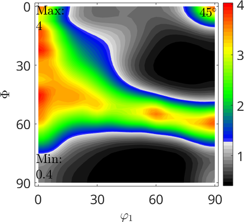
Create Plots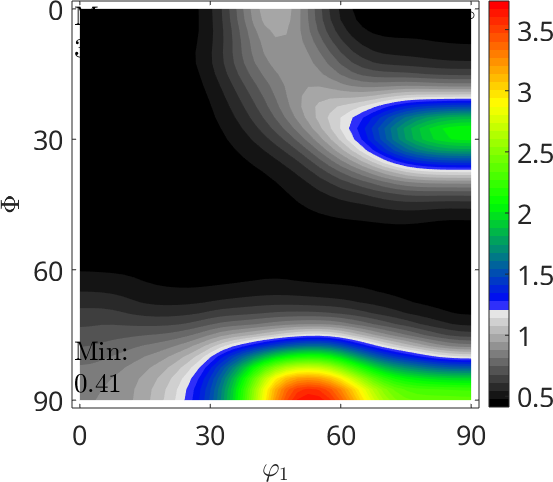
Create Plots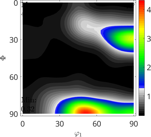
Create Plots

Choose pole figure plot depending on phase
%run('ColorMap4.m')

if strcmp(phase,'austenite')
    pf = calcPoleFigure(odf,h_austenite,cs,ss);
    figure; plotPDF(odf,h_austenite,cs,ss, 'projection','eangle', 'antipodal');setColorRange(gcm,[0, 4]);mtexColorbar;
    %figure; plotPDF(odf,h_austenite,cs,ss, 'antipodal','grid','grid_res',30*degree,'projection','eangle');setColorRange(gcm,[0, 4]);mtexColorbar;

elseif strcmp(phase,'ferrite')
    pf = calcPoleFigure(odf,h_ferrite);
    figure; plotPDF(odf,h_ferrite, cs,ss, 'projection','eangle', 'antipodal');setColorRange(gcm,[0, 4]);mtexColorbar;
else
    'something has gone wrong'
end

% an example script should not litter the repository with image files -
% uncomment to write the figure out
%exportgraphics(gcf,strcat(savepath,filesep,bname,'-PF.tiff'),'Resolution',150)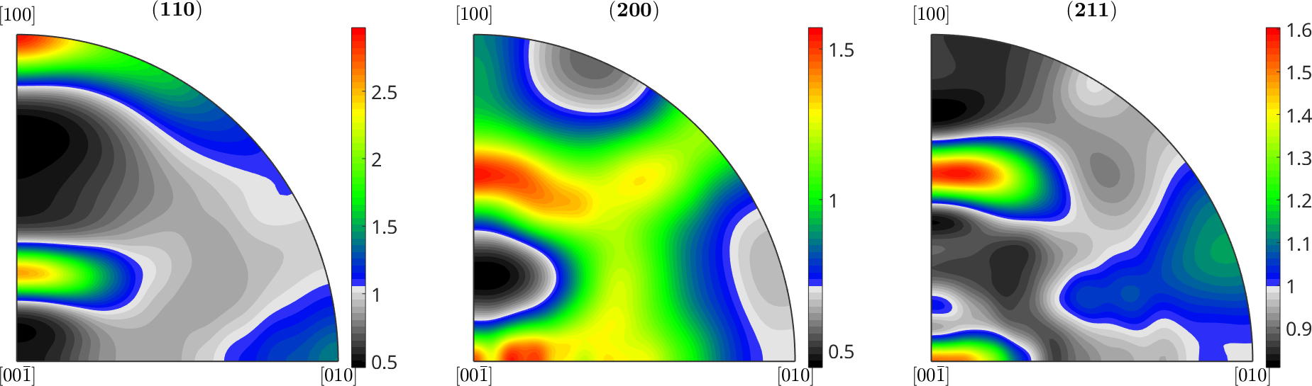
Calculate ODF scalar values and write to file
disp('Calculate ODF scalar values')
%Tval=[textureindex(odf),entropy(odf),max(odf)];
Tval=[textureindex(odf),entropy(odf)];

fileID = fopen(strcat(savepath,'/','ExpTextureValues.txt'),'a');

% Can't output different types of data with the same command
fprintf(fileID,'%12s\t',bname);
fprintf(fileID,'%6.4f\t %6.4f\n',Tval);

fclose(fileID);

%Tval


%odf30 = fibreODF(h,r,ss,'halfwidth',10*degree);
%deg=5*(3.14159)/180;
Calculate ODF scalar values
Warning: The command textureindex is depreciated! Please use squared norm
instead.Calculate ODF scalar values
Warning: The command textureindex is depreciated! Please use squared norm
instead.Calculate ODF scalar values
Warning: The command textureindex is depreciated! Please use squared norm
instead.Calculate ODF scalar values
Warning: The command textureindex is depreciated! Please use squared norm
instead.Commands for output as .maa file
%disp('Output ODFs to .maa and mtex')
disp('Output ODFs to .maa')

arg= cell(1,2);
arg{1}= 'resolution';
arg{2}= degree ;

csplot = crystalSymmetry('m-3m');
ssplot = specimenSymmetry('triclinic');
S3G = getClass(arg,'SO3Grid',regularSO3Grid(csplot,ssplot,arg));

%odf = uniformODF(cs,ss);

v = eval(odf,S3G,arg);

%v = 5*v;

%{

A custom function was created in mtex to save ODFs generated in the .maa format, which is required to import into MAUD.  The .maa format is similar to the popLA data structure (J. S. Kallend, U. F. Kocks, A. D. Rollett, and H.-R. Wenk, “popLA - An Integrated Software System for Texture Analysis,” Textures Microstruct., vol. 14–18, pp. 1203–1208, 1991. ), albeit with whitespace delimited data columns rather than fixed width columns.  While popLA rescaled floating point intensity values an integers (i.e. uniform texture intensity equal to 1.0 was scaled to 100) the .maa format permits floating point numbers.  The function created for .maa output truncates the floating point number to one digit after the decimal point (i.e. ###.#), matching the precision of an .maa file output from MAUD.

%}

file= fopen( strcat(savepath,'/',bname,'.maa'),'w');

% These are boilerplate output for .maa files imported to MAUD
% It looks like these are crystal data, but not used in MAUD
fprintf(file, 'title \n');
fprintf(file, '7 5.0 \n');
fprintf(file, '2.86 2.86 2.86 90.00 90.00 90.00 \n');

%need to add one to the value for Beartex - nope, scale of pole figures
%is still messed up
%between the two programs.  Do we need to rescale?

for i=1:size(v,3)
    for j=1:size(v,2)
       for k=1:size(v,1)
           fprintf(file,'%2.1f ',v(k,j,i));

       end
       fprintf(file,'%2.1f ',v(1,j,i)); %repeat for extra term
       fprintf(file,'  \n');
    end

    fprintf(file,'  \n');
end

%repeat for extra data block
    for j=1:size(v,2)
       for k=1:size(v,1)
           fprintf(file,'%2.1f ',v(k,j,1));

       end
       fprintf(file,'%2.1f ',v(1,j,1));
       fprintf(file,'  \n');
    end
        fprintf(file,'  \n');

%h = {Miller(1,1,0,cs),Miller(2,0,0,cs),Miller(2,1,1,cs)};

%figure
%plotPDF(odf30,h,'contourf',[1.87,1.25,2.5])
%plotPDF(odf,h)
%figure; plotPDF(odf,h,'contourf',[1.0,1.2,1.5,2]);setColorRange(gcm,[0, 2.5]);mtexColorbar;

%setMTEXpref('EulerAngleConvention','ZYZ')
%plot(odf30,'sections',18, 'colorbar')
%setMTEXpref('EulerAngleConvention','Bunge')


% Save Mtex format
%export(odf,strcat(bname,'-mtex.txt'),'resolution',5*degree)

i=i+1;

% close the plots of this data set before moving to the next one. Each pass
% opens several figures and the tiffs above are the output that is wanted,
% so keeping them would just leave a pile of windows behind.
close all

%end of for loop
Output ODFs to .maaOutput ODFs to .maaOutput ODFs to .maaOutput ODFs to .maaend
Citing this page.
This page is part of the documentation of
MTEX, a free and open
source MATLAB toolbox for analyzing and modeling crystallographic textures.
It was written by The MTEX Developers and is published at
https://mtex-toolbox.github.io/ExperimentalPFs.html.
If you use MTEX, or reuse text or figures from this page, in your research,
please cite
F. Bachmann, R. Hielscher, H. Schaeben: Texture Analysis with MTEX - Free and Open Source Software Toolbox, Solid State Phenomena 160 (2010), 63-68. 10.4028/www.scientific.net/SSP.160.63
BibTeX
@article{bachmann2010mtex,
  author  = {F. Bachmann and R. Hielscher and H. Schaeben},
  title   = {Texture Analysis with MTEX - Free and Open Source Software Toolbox},
  journal = {Solid State Phenomena},
  volume  = {160},
  pages   = {63-68},
  year    = {2010},
  doi     = {10.4028/www.scientific.net/SSP.160.63},
  url     = {https://doi.org/10.4028/www.scientific.net/SSP.160.63}
}
Other papers describing specific MTEX methods are listed under Publications — please cite the one that best fits your application. The MTEX source code is licensed under the GNU General Public License v2.0; the text and figures of this documentation are licensed under CC BY 4.0, which permits reuse — including by automated systems — provided The MTEX Developers and this page are credited.