script_CalculatedTexturesPlots edit page

clc
clear
close all

jacPath = fullfile(mtexExamplePath,'JACCreuziger');
run(fullfile(jacPath,'ColorMap4.m'))

cs = crystalSymmetry('m-3m');
ss = specimenSymmetry('orthorhombic');
r = xvector;

% pole figure indexes
%h_ferrite = {Miller(1,1,0,cs),Miller(2,0,0,cs),Miller(2,1,1,cs),Miller(2,2,0,cs),Miller(3,1,0,cs),Miller(2,2,2,cs)} ;
%h_austenite = {Miller(1,1,1,cs),Miller(2,0,0,cs),Miller(2,2,0,cs),Miller(3,1,1,cs),Miller(2,2,2,cs),Miller(4,0,0,cs),Miller(3,3,1,cs),Miller(4,2,0,cs)} ;

% Create save paths (if the don't exist)
AddFiguresDir=fullfile(jacPath,'ODFFigures');
MtexDataDir=fullfile(jacPath,'MtexData');
mkdir(AddFiguresDir)
mkdir(MtexDataDir)

Warning: Directory already exists. 
Warning: Directory already exists.

Define orientations

disp('Define Orientations')

Cube = orientation.byMiller([0 0 1],[1 0 0],cs,ss);
Goss = orientation.byMiller([0 1 1],[1 0 0],cs,ss);
Shear = orientation.byMiller([0 0 1],[1 -1 0],cs,ss);
RGoss = orientation.byEuler(0*degree,90*degree,45*degree,cs,ss);

alpha1=orientation.byMiller([1 1 5],[1 -1 0],cs,ss);
alpha2=orientation.byMiller([1 1 3],[1 -1 0],cs,ss);
alpha3=orientation.byMiller([1 1 2],[1 -1 0],cs,ss);
alpha4=orientation.byMiller([2 2 3],[1 -1 0],cs,ss);

o554=orientation.byMiller([5 5 4],[-2 -2 5],cs,ss);

Copper = orientation.byEuler(90*degree,35.264*degree,45*degree,cs,ss);
CopperS=orientation.byEuler(74.49*degree,35.982*degree,54.2175*degree,cs,ss);
S = orientation.byEuler(58.98*degree,36.699*degree,63.435*degree,cs,ss);
BrassS=orientation.byEuler(47.122*degree,40.85*degree,76.718*degree,cs,ss);
Brass = orientation.byEuler(35.264*degree,45*degree,90*degree,cs,ss);

gamma1 = orientation.byEuler(0*degree,54.736*degree,45*degree,cs,ss);
gamma2 = orientation.byEuler(30*degree,54.736*degree,45*degree,cs,ss);

% Fiber textures are not working properly in mtex when created with fibre()
% command
% Fiber textures will be created by a series of unimodal orientations

Define Orientations

open file to save the Name, texture intex and Entropy

fileID = fopen(fullfile(MtexDataDir,'ComputedTextureIndexValues.txt'),'w');

fprintf(fileID,'%12s\t %5s\t %5s\n','Name','TI', 'Ent');
%fmt = '] ] ] ]\n';
fclose(fileID);

Define kernal and halfwidth %%

%a series of halfwidths is possible, but need to remove comment at end of
%code
%for hw=[10 20 30 40 50]
%for HW=[10*degree 15*degree 20*degree 25*degree 30*degree 35*degree 40*degree 45*degree 50*degree]

%single halfwidth
HW=20*degree;

tmp=num2str(round(HW/degree));
disp(['Halfwidth: ', tmp, ' Degrees'])

disp(HW)
psi = deLaValeePoussinKernel('HALFWIDTH',HW);
%psi = vonMisesFisherKernel('HALFWIDTH',HW);

Halfwidth: 20 Degrees
    0.3491
Warning: The syntax "deLaValeePoussinKernel" is obsolete. Please use
"SO3DeLaValleePoussinKernel" instead.

Start for loop of different orientaions

Define ODFs

for i=1:21

uniform distributions - creates lots of them, but I couldn't find an elegant way to stop that from happening

if i==1
%uniform ODF
        disp('Uniform Austenite')
        bname='UniformA';
        phase ='austenite';
        odf=uniformODF(cs,ss);

elseif i==2

%uniform ODF
        disp('Uniform Ferrite')
        bname='UniformF';
        phase ='ferrite';
        odf=uniformODF(cs,ss);

Uniform Ferrite

fiber distributions

elseif i==3
% ferrite alpha fiber 110 || RD
    bname='AlphaFiberF';
    phase ='ferrite';
    %gamma= fibre.gamma(cs);
    %ah=alphaFiber.h
    %ar=alphaFiber.r
    %odf = fibreODF(Miller(times(ah,o),cs),Miller(times(ar,o),cs),'halfwidth',HW)

    %h = Miller(1,1,0,cs);
    %r = xvector;
    %odf = fibreODF(h,r,ss,psi);
    sixth=(1.0/6.0)
    odf1 = (sixth)*unimodalODF(Shear,'halfwidth',HW,cs,ss,psi);
    odf2 = (sixth)*unimodalODF(alpha1,'halfwidth',HW,cs,ss,psi);
    odf3 = (sixth)*unimodalODF(alpha2,'halfwidth',HW,cs,ss,psi);
    odf4 = (sixth)*unimodalODF(alpha3,'halfwidth',HW,cs,ss,psi);
    odf5 = (sixth)*unimodalODF(alpha4,'halfwidth',HW,cs,ss,psi);
    odf6 = (sixth)*unimodalODF(gamma1,'halfwidth',HW,cs,ss,psi);

    odf=odf1+odf2+odf3+odf4+odf5+odf6;

elseif i==4
% ferrite fiber - gamma 111 || ND
    bname='GammaFiber2F';
    phase ='ferrite';

    odf1=.5*unimodalODF(gamma1,'halfwidth',HW,cs,ss,psi);
    odf2=.5*unimodalODF(gamma2,'halfwidth',HW,cs,ss,psi);
    odf=odf1+odf2;

elseif i==5

% austenite fiber - beta fiber, Brass -> Copper via S
%Not working well using the defined beta fiber in mtex
    phase ='austenite';
    bname='BetaFiberA';

    odf1 = .2*unimodalODF(Brass,'halfwidth',HW,cs,ss);
    odf2 = .2*unimodalODF(S,'halfwidth',HW,cs,ss);
    odf3 = .2*unimodalODF(Copper,'halfwidth',HW,cs,ss);
    odf4 = .2*unimodalODF(CopperS,'halfwidth',HW,cs,ss);
    odf5 = .2*unimodalODF(BrassS,'halfwidth',HW,cs,ss);

    odf=odf1+odf2+odf3+odf4+odf5;

single orientations

% austenite single orientations

elseif i==6
    bname='BrassA';
    phase ='austenite';
    odf = unimodalODF(Brass,'halfwidth',HW,cs,ss);

elseif i==7
    bname='CubeA';
    phase ='austenite';
    odf = unimodalODF(Cube,'halfwidth',HW,cs,ss);

elseif i==8
    bname='CopperA';
    phase ='austenite';
    odf = unimodalODF(Copper,'halfwidth',HW,cs,ss);

elseif i==9
    bname='SA';
    phase ='austenite';
    odf = unimodalODF(S,'halfwidth',HW,cs,ss);

elseif i==10
    bname='GossA';
    phase ='austenite';
    odf = unimodalODF(Goss,'halfwidth',HW,cs,ss);

% ferrite single orientation
elseif i==11
    bname='Gamma1F';
    phase ='ferrite';
    odf = unimodalODF(gamma1,'halfwidth',HW,cs,ss)

elseif i==13
    bname='Gamma2F';
    phase ='ferrite';
    odf = unimodalODF(gamma2,'halfwidth',HW,cs,ss)

elseif i==14
    bname='GossF';
    phase ='ferrite';
    odf = unimodalODF(Goss,'halfwidth',HW,cs,ss)

elseif i==15
    bname='ShearF';
    phase ='ferrite';
    odf = unimodalODF(Shear,'halfwidth',HW,cs,ss)

elseif i==16
    bname='o554F';
    phase ='ferrite';
    odf = unimodalODF(o554,'halfwidth',HW,cs,ss)

elseif i==17
    bname='alpha1F';
    phase ='ferrite';
    odf = unimodalODF(alpha1,'halfwidth',HW,cs,ss)

elseif i==18
    bname='alpha2F';
    phase ='ferrite';
    odf = unimodalODF(alpha2,'halfwidth',HW,cs,ss)

elseif i==19
    bname='alpha3F';
    phase ='ferrite';
    odf = unimodalODF(alpha3,'halfwidth',HW,cs,ss)

elseif i==20
    bname='alpha4F';
    phase ='ferrite';
    odf = unimodalODF(alpha4,'halfwidth',HW,cs,ss)

elseif i==21
    bname='RGossF';
    phase ='ferrite';
    odf = unimodalODF(RGoss,'halfwidth',HW,cs,ss)


end

Uniform Austenite

sixth =
    0.1667

odf = SO3FunRBF (m3̅m → y↓→x (mmm))
 
  unimodal component
  kernel: de la Vallee Poussin, halfwidth 20°
  center: 1 orientations
 
  Bunge Euler angles in degree
  phi1    Phi   phi2 weight
     0 54.736     45      1

odf = SO3FunRBF (m3̅m → y↓→x (mmm))
 
  unimodal component
  kernel: de la Vallee Poussin, halfwidth 20°
  center: 1 orientations
 
  Bunge Euler angles in degree
  phi1    Phi   phi2 weight
    30 54.736     45      1

odf = SO3FunRBF (m3̅m → y↓→x (mmm))
 
  unimodal component
  kernel: de la Vallee Poussin, halfwidth 20°
  center: 1 orientations
 
  Bunge Euler angles in degree
  phi1    Phi   phi2 weight
     0     45      0      1

odf = SO3FunRBF (m3̅m → y↓→x (mmm))
 
  unimodal component
  kernel: de la Vallee Poussin, halfwidth 20°
  center: 1 orientations
 
  Bunge Euler angles in degree
  phi1    Phi   phi2 weight
    45      0      0      1

odf = SO3FunRBF (m3̅m → y↓→x (mmm))
 
  unimodal component
  kernel: de la Vallee Poussin, halfwidth 20°
  center: 1 orientations
 
  Bunge Euler angles in degree
  phi1     Phi    phi2  weight
   270 60.5038      45       1

odf = SO3FunRBF (m3̅m → y↓→x (mmm))
 
  unimodal component
  kernel: de la Vallee Poussin, halfwidth 20°
  center: 1 orientations
 
  Bunge Euler angles in degree
  phi1     Phi    phi2  weight
     0 15.7932      45       1

odf = SO3FunRBF (m3̅m → y↓→x (mmm))
 
  unimodal component
  kernel: de la Vallee Poussin, halfwidth 20°
  center: 1 orientations
 
  Bunge Euler angles in degree
  phi1     Phi    phi2  weight
     0 25.2394      45       1

odf = SO3FunRBF (m3̅m → y↓→x (mmm))
 
  unimodal component
  kernel: de la Vallee Poussin, halfwidth 20°
  center: 1 orientations
 
  Bunge Euler angles in degree
  phi1     Phi    phi2  weight
     0 35.2644      45       1

odf = SO3FunRBF (m3̅m → y↓→x (mmm))
 
  unimodal component
  kernel: de la Vallee Poussin, halfwidth 20°
  center: 1 orientations
 
  Bunge Euler angles in degree
  phi1     Phi    phi2  weight
     0 43.3139      45       1

odf = SO3FunRBF (m3̅m → y↓→x (mmm))
 
  unimodal component
  kernel: de la Vallee Poussin, halfwidth 20°
  center: 1 orientations
 
  Bunge Euler angles in degree
  phi1    Phi   phi2 weight
     0     90     45      1

Create Plots

disp('Create Plots')

figure;
plot(odf,'phi2',[45]*degree,'projection','plain','silent',cs,ss,'FontSize',20);
setColorRange(gcm,[0, 4]);
mtexColorbar;
fig = gcf;
fig.PaperPositionMode = 'auto';
% an example script should not litter the repository with image files -
% uncomment to write the figure out
%saveas(fig,fullfile(AddFiguresDir,strcat(bname,'-HW', tmp,'-phi2ODF.png')))


%saveas(fig,fullfile(AddFiguresDir,strcat(bname,'-HW', tmp,'-phi2ODF.png')))

%gcf=plot(alpha1F,'phi2',[45]*degree,'projection','plain','silent',cs,ss,'FontSize',20)
%fig = gcf;





%figure; plot(odf,'phi2',[45]*degree,'projection','plain','silent',cs,ss,'FontSize',20);setColorRange(gcm,[0, 4]);mtexColorbar;
%export_fig(strcat(savepath,'/',bname,'-phi2-45ODF.png'),'-r300')


%ODF plot
%figure; plot(odf,'phi2','sections',18,'projection','plain','minmax', 'off',cs,ss);setColorRange(gcm,[0, 4]);mtexColorbar;
%fig = gcf;
%fig.PaperPositionMode = 'auto';
%saveas(fig,fullfile(AddFiguresDir,strcat(bname,'-HW', tmp,'-phi2ODF.png')))

%Save 45 cross section

Create Plots

Create Plots

Create Plots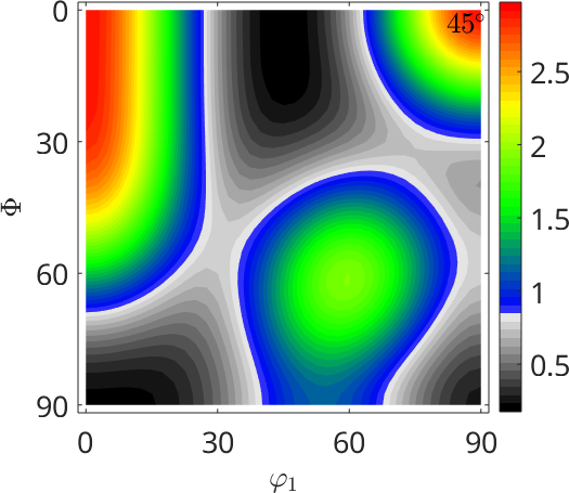

Create Plots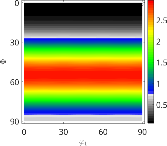

Create Plots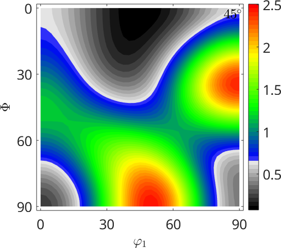

Create Plots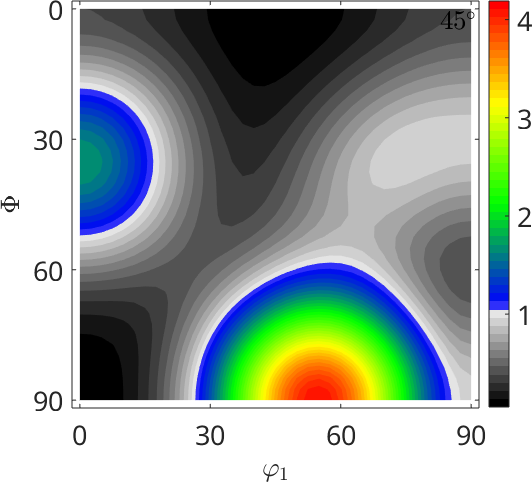

Create Plots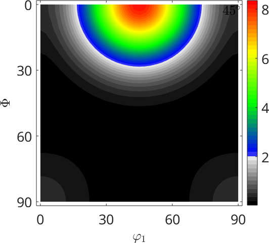

Create Plots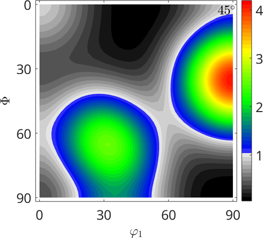

Create Plots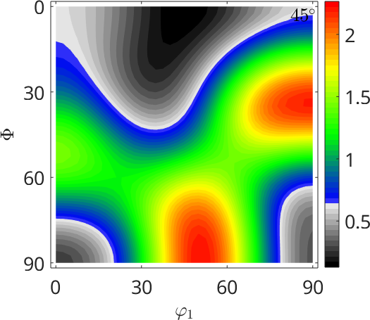

Create Plots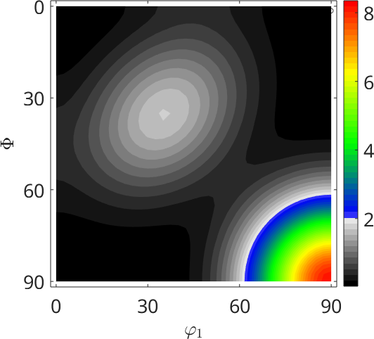

Create Plots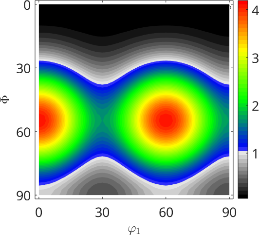

Create Plots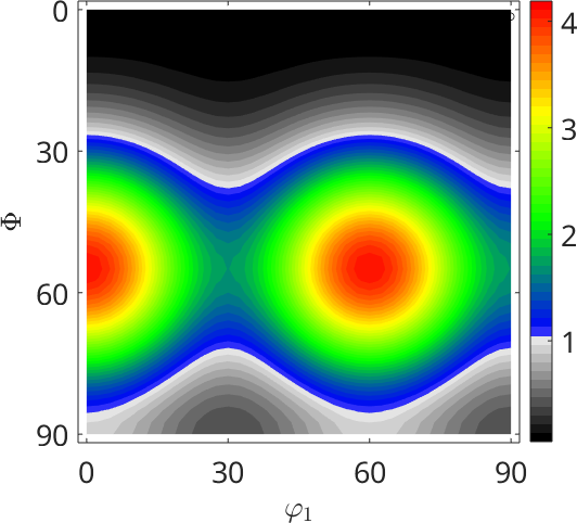

Create Plots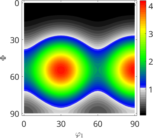

Create Plots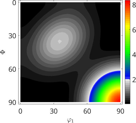

Create Plots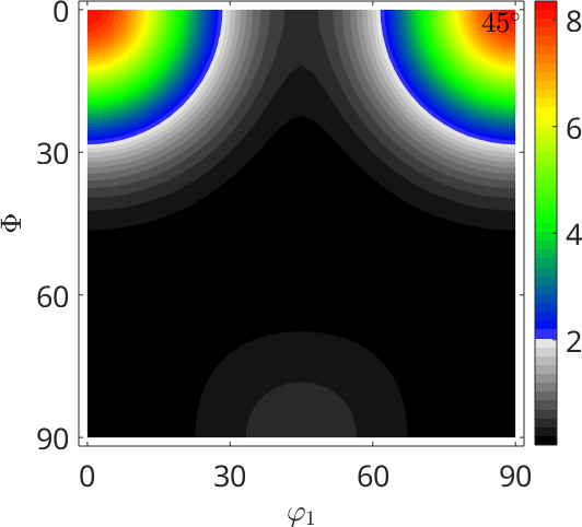

Create Plots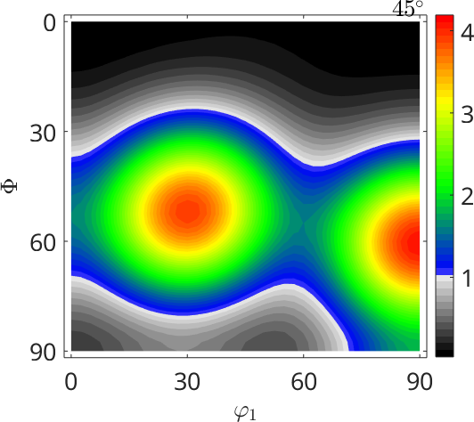

Create Plots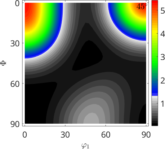

Create Plots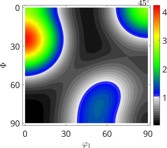

Create Plots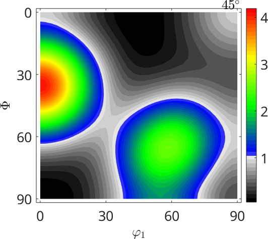

Create Plots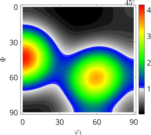

Create Plots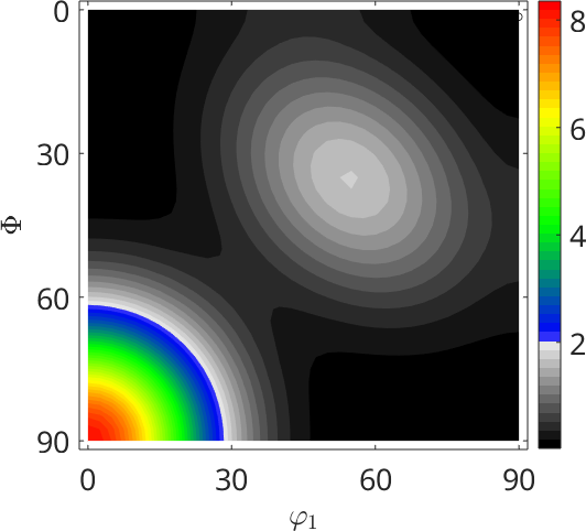

Calculate ODF scalar values and write to file

disp('Calculate ODF scalar values')
%Tval=[textureindex(odf),entropy(odf),max(odf)];

Tval=[textureindex(odf),entropy(odf)];


fileID = fopen(fullfile(MtexDataDir,'ComputedTextureIndexValues.txt'),'a');
% Can't output different types of data with the same command
fprintf(fileID,'%12s\t',bname);
fprintf(fileID,'%6.4f\t %6.4f\n',Tval);

fclose(fileID);

%Tval


%odf30 = fibreODF(h,r,ss,'halfwidth',10*degree);
%deg=5*(3.14159)/180;

Calculate ODF scalar values
Warning: The command textureindex is depreciated! Please use squared norm
instead.

Calculate ODF scalar values
Warning: The command textureindex is depreciated! Please use squared norm
instead.

Calculate ODF scalar values
Warning: The command textureindex is depreciated! Please use squared norm
instead.

Calculate ODF scalar values
Warning: The command textureindex is depreciated! Please use squared norm
instead.

Calculate ODF scalar values
Warning: The command textureindex is depreciated! Please use squared norm
instead.

Calculate ODF scalar values
Warning: The command textureindex is depreciated! Please use squared norm
instead.

Calculate ODF scalar values
Warning: The command textureindex is depreciated! Please use squared norm
instead.

Calculate ODF scalar values
Warning: The command textureindex is depreciated! Please use squared norm
instead.

Calculate ODF scalar values
Warning: The command textureindex is depreciated! Please use squared norm
instead.

Calculate ODF scalar values
Warning: The command textureindex is depreciated! Please use squared norm
instead.

Calculate ODF scalar values
Warning: The command textureindex is depreciated! Please use squared norm
instead.

Calculate ODF scalar values
Warning: The command textureindex is depreciated! Please use squared norm
instead.

Calculate ODF scalar values
Warning: The command textureindex is depreciated! Please use squared norm
instead.

Calculate ODF scalar values
Warning: The command textureindex is depreciated! Please use squared norm
instead.

Calculate ODF scalar values
Warning: The command textureindex is depreciated! Please use squared norm
instead.

Calculate ODF scalar values
Warning: The command textureindex is depreciated! Please use squared norm
instead.

Calculate ODF scalar values
Warning: The command textureindex is depreciated! Please use squared norm
instead.

Calculate ODF scalar values
Warning: The command textureindex is depreciated! Please use squared norm
instead.

Calculate ODF scalar values
Warning: The command textureindex is depreciated! Please use squared norm
instead.

Calculate ODF scalar values
Warning: The command textureindex is depreciated! Please use squared norm
instead.

Calculate ODF scalar values
Warning: The command textureindex is depreciated! Please use squared norm
instead.

Commands for output

%disp('Output ODFs to .maa and mtex')
disp('Output ODFs to .maa')

arg= cell(1,2);
arg{1}= 'resolution';
arg{2}= degree ;

csplot = crystalSymmetry('m-3m');
ssplot = specimenSymmetry('triclinic');
S3G = getClass(arg,'SO3Grid',regularSO3Grid(csplot,ssplot,arg));

%odf = uniformODF(cs,ss);

v = eval(odf,S3G,arg);

%v = 5*v;

%{

A custom function was created in mtex to save ODFs generated in the .maa format, which is required to import into MAUD.  The .maa format is similar to the popLA data structure (J. S. Kallend, U. F. Kocks, A. D. Rollett, and H.-R. Wenk, “popLA - An Integrated Software System for Texture Analysis,” Textures Microstruct., vol. 14–18, pp. 1203–1208, 1991. ), albeit with whitespace delimited data columns rather than fixed width columns.  While popLA rescaled floating point intensity values an integers (i.e. uniform texture intensity equal to 1.0 was scaled to 100) the .maa format permits floating point numbers.  The function created for .maa output truncates the floating point number to one digit after the decimal point (i.e. ###.#), matching the precision of an .maa file output from MAUD.


%}

file= fopen( strcat(MtexDataDir,'/',bname,'.maa'),'w');

fprintf(file, 'title \n');
fprintf(file, '7 5.0 \n'); % angle convention and resolution
fprintf(file, '2.86 2.86 2.86 90.00 90.00 90.00 \n');% This is generic header information, not specfic to each phase



for i=1:size(v,3)
    for j=1:size(v,2)
       for k=1:size(v,1)
           fprintf(file,'%2.1f ',v(k,j,i));

       end
       fprintf(file,'%2.1f ',v(1,j,i)); %repeat for extra term
       fprintf(file,'  \n');
    end

    fprintf(file,'  \n');
end

%repeat for extra data block
    for j=1:size(v,2)
       for k=1:size(v,1)
           fprintf(file,'%2.1f ',v(k,j,1));

       end
       fprintf(file,'%2.1f ',v(1,j,1));
       fprintf(file,'  \n');
    end
        fprintf(file,'  \n');

%h = {Miller(1,1,0,cs),Miller(2,0,0,cs),Miller(2,1,1,cs)};

%figure
%plotPDF(odf30,h,'contourf',[1.87,1.25,2.5])
%plotPDF(odf,h)
%figure; plotPDF(odf,h,'contourf',[1.0,1.2,1.5,2]);setColorRange(gcm,[0, 2.5]);mtexColorbar;

%setMTEXpref('EulerAngleConvention','ZYZ')
%plot(odf30,'sections',18, 'colorbar')
%setMTEXpref('EulerAngleConvention','Bunge')


% Save Mtex format
%export(odf,strcat(bname,'-mtex.txt'),'resolution',5*degree)

i=i+1;

close all

Output ODFs to .maa

Output ODFs to .maa

Output ODFs to .maa

Output ODFs to .maa

Output ODFs to .maa

Output ODFs to .maa

Output ODFs to .maa

Output ODFs to .maa

Output ODFs to .maa

Output ODFs to .maa

Output ODFs to .maa

Output ODFs to .maa

Output ODFs to .maa

Output ODFs to .maa

Output ODFs to .maa

Output ODFs to .maa

Output ODFs to .maa

Output ODFs to .maa

Output ODFs to .maa

Output ODFs to .maa

Output ODFs to .maa

end








% end halfwidth loop
%end

Citing this page. This page is part of the documentation of MTEX, a free and open source MATLAB toolbox for analyzing and modeling crystallographic textures. It was written by The MTEX Developers and is published at https://mtex-toolbox.github.io/CalculatedTexturesPlots.html. If you use MTEX, or reuse text or figures from this page, in your research, please cite

F. Bachmann, R. Hielscher, H. Schaeben: Texture Analysis with MTEX - Free and Open Source Software Toolbox, Solid State Phenomena 160 (2010), 63-68. 10.4028/www.scientific.net/SSP.160.63

BibTeX

@article{bachmann2010mtex,
  author  = {F. Bachmann and R. Hielscher and H. Schaeben},
  title   = {Texture Analysis with MTEX - Free and Open Source Software Toolbox},
  journal = {Solid State Phenomena},
  volume  = {160},
  pages   = {63-68},
  year    = {2010},
  doi     = {10.4028/www.scientific.net/SSP.160.63},
  url     = {https://doi.org/10.4028/www.scientific.net/SSP.160.63}
}

Other papers describing specific MTEX methods are listed under Publications — please cite the one that best fits your application. The MTEX source code is licensed under the GNU General Public License v2.0; the text and figures of this documentation are licensed under CC BY 4.0, which permits reuse — including by automated systems — provided The MTEX Developers and this page are credited.