In this section we discuss parent grain reconstruction at the example of a titanium alloy. Lets start by importing a sample data set
mtexdata alphaBetaTitanium
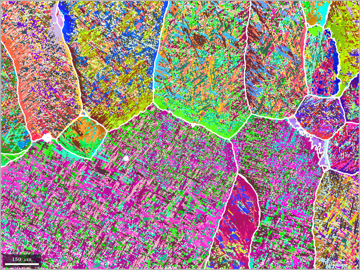
% and plot the alpha phase as an inverse pole figure map
plot(ebsd('Ti (alpha)'),ebsd('Ti (alpha)').orientations,'figSize','large')ebsd = EBSD
Phase Orientations Mineral Color Symmetry Crystal reference frame
0 10449 (5.3%) notIndexed
1 437 (0.22%) Ti (BETA) LightSkyBlue 432
2 185722 (94%) Ti (alpha) DarkSeaGreen 622 X||a*, Y||b, Z||c*
Properties: bands, bc, bs, error, mad, reliabilityindex, x, y
Scan unit : um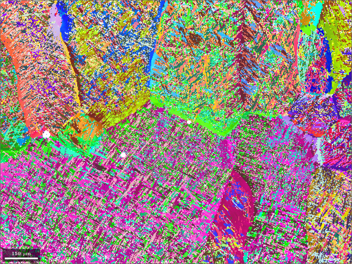
The data set contains 99.8 percent alpha titanium and 0.2 percent beta titanium. Our goal is to reconstuct the original beta phase. The original grain structure appears almost visible for human eyes. Our computations will be based on the Burgers orientation relationship
beta2alpha = orientation.Burgers(ebsd('Ti (beta)').CS,ebsd('Ti (alpha)').CS)beta2alpha = misorientation (Ti (BETA) → Ti (alpha))
(110) || (0001) [1-11] || [-2110]that alligns (110) plane of the beta phase with the (0001) plane of the alpha phase and the [1-11] direction of the beta phase with the [-2110] direction of the alpha phase.
Note that all MTEX functions for parent grain reconstruction expect the orientation relationship as parent to child and not as child to parent.
Setting up the parent grain reconstructor
Grain reconstruction is guided in MTEX by a variable of type parentGrainReconstructor. During the reconstruction process this class keeps track about the relationship between the measured child grains and the recovered parent grains. In order to set this variable up we first need to compute the initital child grains from out EBSD data set.
% reconstruct grains
[grains,ebsd.grainId] = calcGrains(ebsd('indexed'),'threshold',1.5*degree);
We choose a very small threshold of 1.5 degree for the identification of grain boundaries to avoid alpha orientations that belong to different beta grains get merged into the same alpha grain.
Now we are ready to set up the parent grain reconstruction job.
job = parentGrainReconstructor(ebsd, grains);
job.p2c = beta2alpha
job = parentGrainReconstructor
phase mineral symmetry grains area reconstructed
parent Ti (BETA) 432 432 0.23% 0%
child Ti (alpha) 622 61115 100%
OR: (110) || (0001) [1-11] || [-2110]
p2c fit: 0.82°, 1.2°, 1.6°, 3.1° (quintiles)
c2c fit: 0.71°, 0.99°, 1.3°, 1.7° (quintiles)The output of the job variable allows you to keep track of the amount of already recovered parent grains. Using the variable job you have access to the following properties
job.grainsIn- the input grainsjob.grains- the grains at the current stage of reconstructionjob.ebsdIn- the input EBDS datajob.ebsd- the ebsd data at the current stage of reconstructionjob.mergeId- the relationship between the input grainsjob.grainsInand the current grainsjob.grains, i.e.,job.grainsIn(ind)goes into the merged grainjob.grains(job.mergeId(ind))job.numChilds- number of childs of each current parent grainjob.parenGrains- the current parent grainsjob.childGrains- the current child grainsjob.isTransformed- which of thegrainsMeasuredhave a computed parentjob.isMerged- which of thegrainsMeasuredhave been merged into a parent grainjob.transformedGrains- child grains ingrainsMeasuredwith computed parent grain
Additionaly, the parentGrainReconstructor class provides the following operations for parent grain reconstruction. These operators can be applied multiple times and in any order to archieve the best possible reconstruction.
job.calcVariantGraph- compute the variant graphjob.clusterVariantGraph- compute votes from the variant graphjob.calcGBVotes- detect child/child and parent/child grain boundariesjob.calcTPVotes- detect child/child/child triple pointsjob.calcParentFromVote- recover parent grains from votesjob.calcParentFromGraph- recover parent grains from graph clusteringjob.mergeSimilar- merge similar parent grainsjob.mergeInclusions- merge inclusions
The main line of the variant graph based reconstruction algorithm is as follows. First we compute the variant graph using the command job.calcVariantGraph
job.calcVariantGraph('threshold',1.5*degree)ans = parentGrainReconstructor
phase mineral symmetry grains area reconstructed
parent Ti (BETA) 432 432 0.23% 0%
child Ti (alpha) 622 61115 100%
OR: (110) || (0001) [1-11] || [-2110]
p2c fit: 0.82°, 1.2°, 1.6°, 3.1° (quintiles)
c2c fit: 0.71°, 1°, 1.3°, 1.7° (quintiles)
variant graph: 615123 entriesIn a second step we cluster the variant graph and at the same time compute probabilites for potential parent orientations using the command job.clusterVariantGraph
job.clusterVariantGraph('numIter',3)ans = parentGrainReconstructor
phase mineral symmetry grains area reconstructed
parent Ti (BETA) 432 432 0.23% 0%
child Ti (alpha) 622 61115 100%
OR: (110) || (0001) [1-11] || [-2110]
p2c fit: 0.82°, 1.2°, 1.6°, 3.1° (quintiles)
c2c fit: 0.72°, 0.99°, 1.3°, 1.7° (quintiles)
votes: 61115 x 1
probabilities: 100%, 99%, 96%, 88% (quintiles)The probabilities are stored in job.votes.prob and the corresponding variant ids in job.votes.parentId. In order to use the parent orientation with the highest probability for the reconstruction we use the command job.calcParentFromVote
job.calcParentFromVoteans = parentGrainReconstructor
phase mineral symmetry grains area reconstructed
parent Ti (BETA) 432 59721 99% 97%
child Ti (alpha) 622 1826 1.1%
OR: (110) || (0001) [1-11] || [-2110]
p2c fit: 3.1°, 25°, 35°, 42° (quintiles)
c2c fit: 2.2°, 5°, 12°, 19° (quintiles)
votes: 1826 x 1
probabilities: 0%, 0%, 0%, 0% (quintiles)We observe that after this step more then 99 percent of the grains became parent grains. Lets visualize these reconstructed beta grains
% define a color key
ipfKey = ipfColorKey(ebsd('Ti (Beta)'));
ipfKey.inversePoleFigureDirection = vector3d.Y;

% plot the result
color = ipfKey.orientation2color(job.parentGrains.meanOrientation);
plot(job.parentGrains, color, 'figSize', 'large')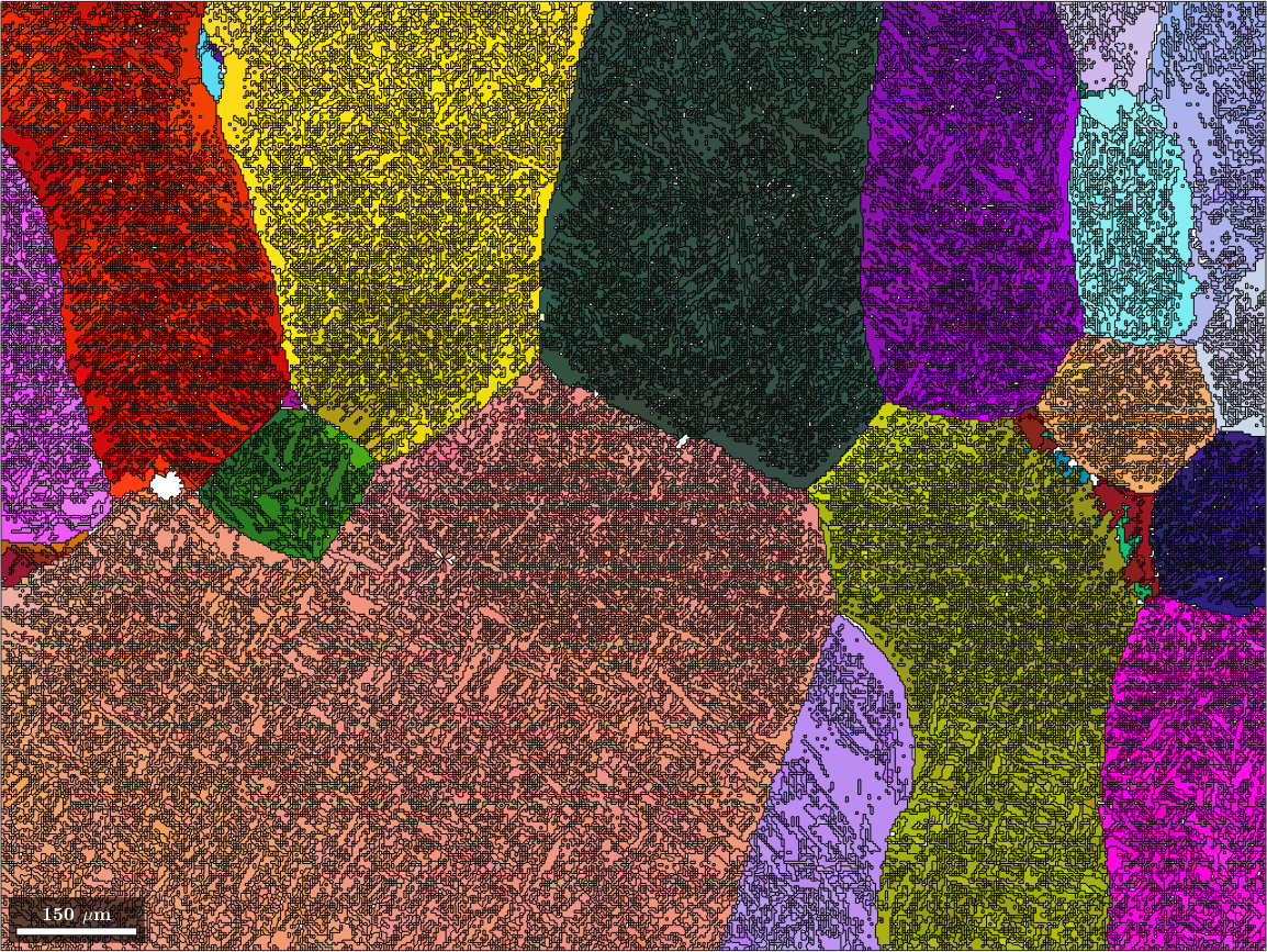
Merge parent grains
After the previous steps we are left with many very similar parent grains. In order to merge all similarly oriented grains into large parent grains one can use the command mergeSimilar. It takes as an option the threshold below which two parent grains should be considered a a single grain.
job.mergeSimilar('threshold',5*degree)

% plot the result
color = ipfKey.orientation2color(job.parentGrains.meanOrientation);
plot(job.parentGrains, color, 'figSize', 'large')
ans = parentGrainReconstructor
phase mineral symmetry grains area reconstructed
parent Ti (BETA) 432 122 99% 97%
child Ti (alpha) 622 1786 1.1%
OR: (110) || (0001) [1-11] || [-2110]
p2c fit: 3.2°, 19°, 34°, 41° (quintiles)
c2c fit: 4.5°, 9.4°, 17°, 23° (quintiles)
votes: 1826 x 1
probabilities: 0%, 0%, 0%, 0% (quintiles)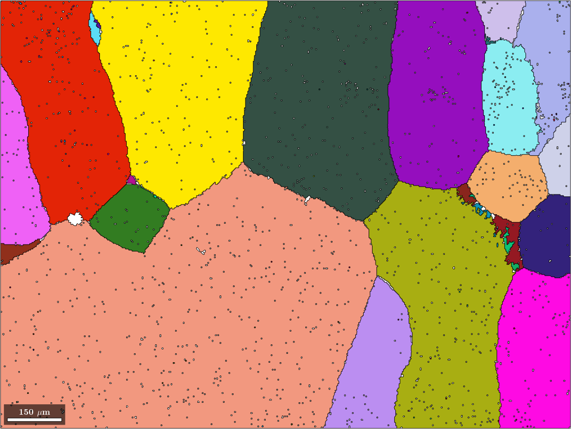
Merge inclusions
We may be still a bit unsatisfied with the result as the large parent grains contain a lot of poorly indexed inclusions where we failed to assign a parent orientation. We use the command mergeInclusions to merge all inclusions that have fever pixels then a certain threshold into the surrounding parent grains.
job.mergeInclusions('maxSize',10)

% plot the result
color = ipfKey.orientation2color(job.parentGrains.meanOrientation);
plot(job.parentGrains, color, 'figSize', 'large')
ans = parentGrainReconstructor
phase mineral symmetry grains area reconstructed
parent Ti (BETA) 432 40 100% 100%
child Ti (alpha) 622 261 0.21%
OR: (110) || (0001) [1-11] || [-2110]
p2c fit: 3.3°, 6°, 18°, 32° (quintiles)
c2c fit: 4.8°, 8.3°, 15°, 20° (quintiles)
votes: 1826 x 1
probabilities: 0%, 0%, 0%, 0% (quintiles)
Reconstruct beta orientations in EBSD map
Until now we have only recovered the beta orientations as the mean orientations of the beta grains. In this section we want to set up the EBSD variable parentEBSD to contain for each pixel a reconstruction of the parent phase orientation. This is done by the command calcParentEBSD
parentEBSD = job.ebsd;

% plot the result
color = ipfKey.orientation2color(parentEBSD('Ti (Beta)').orientations);
plot(parentEBSD('Ti (Beta)'),color,'figSize','large')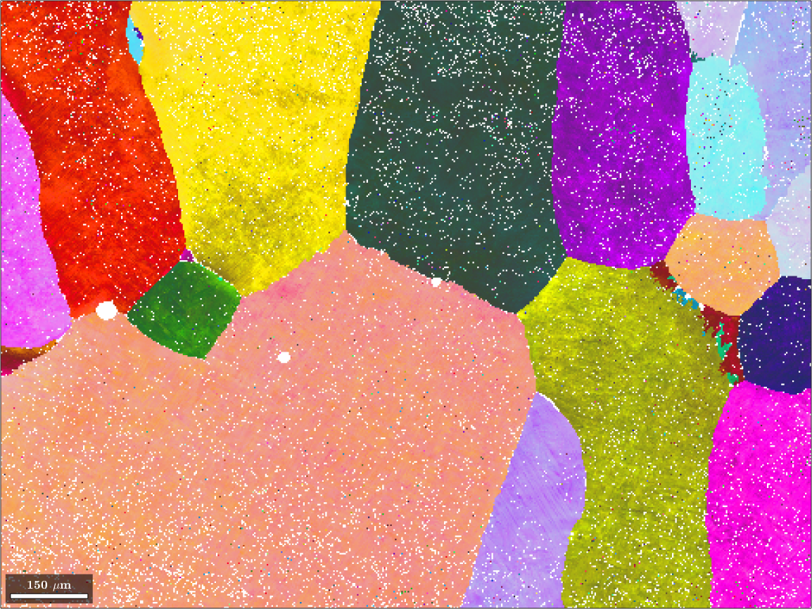
The recovered EBSD variable parentEBSD contains a measure parentEBSD.fit for the corespondence between the beta orientation reconstructed for a single pixel and the beta orientation of the grain. Lets visualize this
% the beta phase
plot(parentEBSD, parentEBSD.fit ./ degree,'figSize','large')
mtexColorbar
setColorRange([0,5])
mtexColorMap('LaboTeX')

hold on
plot(job.grains.boundary,'lineWidth',2)
hold off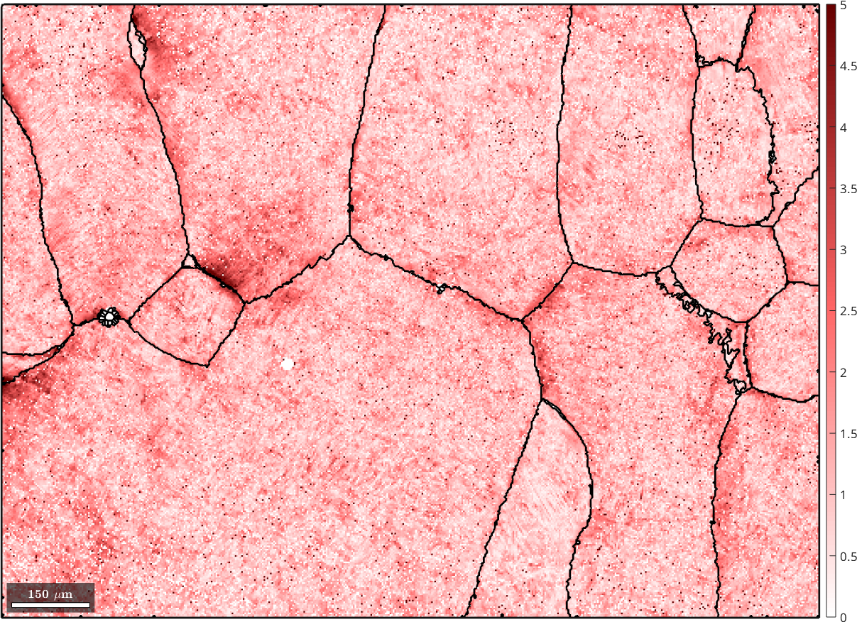
For comparison the map with original alpha phase and on top the recovered beta grain boundaries
plot(ebsd('Ti (Alpha)'),ebsd('Ti (Alpha)').orientations,'figSize','large')

hold on
parentGrains = smooth(job.grains,5);
plot(parentGrains.boundary,'lineWidth',3,'lineColor','White')
hold off